 Material to support teaching in Environmental Science at The University of Western Australia
Units ENVT3361, ENVT4461, and ENVT5503
Time Series Analysis
Concepts using soil temperature data
Andrew Rate
2025-12-09
This guide is organised into 3 main sections:
Set up the R environment for time series analysis
We will need the additional functions in several R packages for specialized time series and other functions in R...
# Load the packages we need
library(zoo)      # for basic irregular time series functions
library(xts)      # we need the xts "eXtended Time Series" format for some functions
library(Kendall)  # for trend analysis with Mann-Kendall test
library(trend)    # for trend analysis using the Sen slope
library(forecast) # for time series forecasting with ARIMA and exponential smoothing
library(tseries)  # for assessing stationarity using Augmented Dickey-Fuller test
library(lmtest)   # for Breusch-Pagan heteroscedasticity test etc.
library(car)      # for various commonly-used functions
library(viridis)  # accessible colour palettes
library(ggplot2)  # alternative to base R plots

# (optional) make a better colour palette than the R default!
# (using viridis package for accessibility e.g. colourblindness)
palette(c("black", plasma(4, end=0.5),plasma(4, alpha=0.5, begin=0.5),"white",
          "darkgray"))
par(mfrow=c(3,1), mar=c(4,4,1,1), mgp=c(1.7,0.3,0), tcl=0.25, font.lab=2)
1. How R reads and stores time series data
We first read the data into a data frame – this is how R
often stores data – it's not the format we need, but we'll use it for
comparison.
The data used are derived from autumn 2014 soil meteorological observations at the Murrumbidgee M2 (Canberra Airport) site, available in the OzNet data archive, and described by Smith et al. (2012).
Non-time series object for comparison
git <- "https://raw.githubusercontent.com/Ratey-AtUWA/Learn-R-web/main/"
soiltemp <- read.csv(paste0(git,"soiltemp2.csv"))
colnames(soiltemp) <- c("Date","temp")
Do some checks of the (non-time series) data
summary(soiltemp) # simple summary of each column
str(soiltemp) # more detailed information about the R object
# ('str'=structure, i.e. how the data are organised in the R object)
## Date temp
## Length:1464 Min. :10.40
## Class :character 1st Qu.:12.45
## Mode :character Median :14.30
## Mean :14.86
## 3rd Qu.:17.41
## Max. :21.70
## 'data.frame': 1464 obs. of 2 variables:
## $ Date: chr "2014-04-01 00:00:00" "2014-04-01 01:00:00" "2014-04-01 02:00:00" "2014-04-01 03:00:00" ...
## $ temp: num 20.1 19.8 19.6 19.2 19 ...
We can also check the general form of the data with a plot (Figure
1). From this plot and from the text summary output above, we can see
that the Date column is not a date or time, or even
numeric.
par(mfrow = c(1,1), mar = c(3,3,1,1), mgp=c(1.6,0.3,0), tcl=0.25, oma = c(0,0,0,0), font.lab=2)
with(soiltemp, plot(temp, type = "l", col = 11))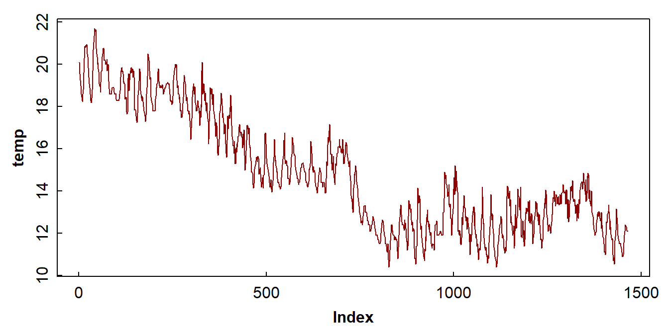
Figure 1: Plot of soil temperature time series data which is not (yet) formatted as a time series.
Reading and storing data as time series
We really want the data in a different type of R object! We use the
read.csv.zoo() function from the zoo package
to read the data in as a time series. This gives a data
object of class zoo which is much more flexible than the
default time series object in R.
We need to specify a format that our date/time information is stored
as. The character string "%Y-%m-%d %H:%M:%S" looks unusual
but it should make sense (%Y is 4-digit year, and so on).
If we have opened and saved our .csv file in Excel, the
format will probably change, so we should try
format = "%d/%m/%Y %H:%M:%S". If in doubt, try to match the
format win the actual .csv file.
soiltemp_T15_zoo <- read.csv.zoo(paste0(git,"soiltemp2.csv"),
                               format = "%Y-%m-%d %H:%M:%S",
                               tz = "Australia/Perth",
                               index.column=1,
                               header = TRUE)
# do some quick checks of the new R object:
summary(soiltemp_T15_zoo) ; cat("\n")
str(soiltemp_T15_zoo) # POSIXct in the output is a date-time format
## Index soiltemp_T15_zoo
## Min. :2014-04-01 00:00:00 Min. :10.40
## 1st Qu.:2014-04-16 05:45:00 1st Qu.:12.45
## Median :2014-05-01 11:30:00 Median :14.30
## Mean :2014-05-01 11:30:00 Mean :14.86
## 3rd Qu.:2014-05-16 17:15:00 3rd Qu.:17.41
## Max. :2014-05-31 23:00:00 Max. :21.70
##
## 'zoo' series from 2014-04-01 to 2014-05-31 23:00:00
## Data: num [1:1464] 20.1 19.8 19.6 19.2 19 ...
## Index: POSIXct[1:1464], format: "2014-04-01 00:00:00" "2014-04-01 01:00:00" "2014-04-01 02:00:00" ...We can see that the column Date has now become
Index, and it's correctly stored as date/time information,
in a format called POSIXct (for more information, run
?DateTimeClasses in the Console. Again, it's usually useful
to check our data with a plot (Figure 2).
par(mfrow=c(1,1), mar=c(3,3,1,1), mgp=c(1.6,0.3,0), tcl=0.25, font.lab=2)
plot(soiltemp_T15_zoo, col = 3) 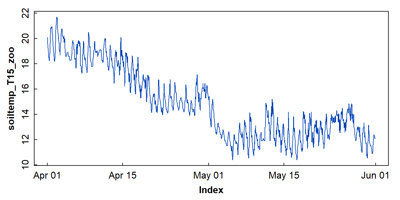
Figure 2: Plot of soil temperature time series data which is formatted as a zoo time series object.
Sometimes we need to use another time series data format,
xts (eXtended Time Series), which
allows us to use more functions...
2. Exploratory data analysis and decomposition of time series
This section is designed to help you understand the features and components of time series, and some of the statistical methods that we use to analyse them. We also look at time series decomposition. The important issues are:
- Do we need to transform our time series variable?
- Is our time series stationary?
- Can we separate out a trend in out variable vs. time?
- Is our time series seasonal (periodic) and, if so, what is the periodic frequency?
- Is there significant autocorrelation in our data?
- What is left unexplained after we isolate the trend and periodicity?
Not all of these would need to be presented in a Report, but it's useful for us to understand time series concepts. This is especially true for autocorrelation and moving averages, which both rely [at least partially] on past observations to estimate current observations. From there it follows that we may be able to use past observations to predict future observations – i.e., forecasting.
We first examine a plot of the data in our time series object (the
plot for the xts time series object is in Figure 3).
par(mfrow=c(1,1), mar=c(3,3,1,1), mgp=c(1.6,0.3,0), tcl=0.25, font.lab=2)
plot(soiltemp_T15_xts, col = 3, ylab = "Soil temperature (\u00B0C)") # just to check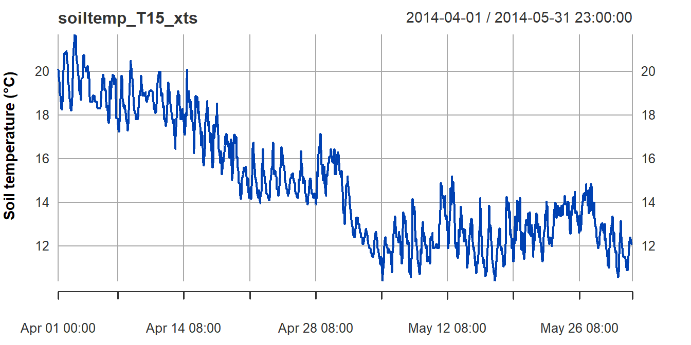
Figure 3: Plot of soil temperature time series data which is formatted
as an xts time series object.
Plotting the time series variable (with time as the independent
variable!) can give us some initial clues about the overall trend in the
data (in Figure 3, a negative overall slope) and if there is any
periodicity (there do seem to be regular increases and decreases in soil
temperature). The plot in Figure 3 also shows that plotting an
xts time series object gives a somewhat more detailed plot
than for a zoo formatted time series object (Figure 2).
We often want to inspect plots of both the raw data and using common transformations (Figure 4). We compare with transformed time series data – we may need to do this to meet later modelling assumptions.
First we change the default plotting parameters using
par(...), then plot the object and some transformed
versions (with custom axis labels).
plot(soiltemp_T15_zoo, ylab = "Temperature (\u00B0C)",
     xlab = "Date", col = 2, lwd = 2, cex.lab = 1.4)
mtext("Untransformed", side=3, line=-1.5, col=2, adj=0.98, font=2)
plot(log10(soiltemp_T15_zoo),
     ylab = expression(bold(paste(log[10],"(Temperature, \u00B0C)"))),
     xlab = "Date", col = 4, lwd = 2, cex.lab = 1.4)
mtext("log-transformed", side=3, line=-1.5, col=4, adj=0.98, font=2)
pt0 <- powerTransform(coredata(soiltemp_T15_zoo))
if(pt0$lambda<0) {
  plot(
    -1 * (soiltemp_T15_zoo ^ pt0$roundlam), # use rounded power term
    ylab = "power-transf. (Temp., \u00B0C)",
    xlab = "Date",
    col = 5, lwd = 2, cex.lab = 1.4
  )
} else {
  plot((soiltemp_T15_zoo ^ pt0$roundlam), # use rounded power term
       ylab = "power-transf. (Temp., \u00B0C)",
       xlab = "Date",
       col = 5, lwd = 2, cex.lab = 1.4
  )
}
mtext("power-transformed", side=3, line=-1.5, col=5, adj=0.98, font=2)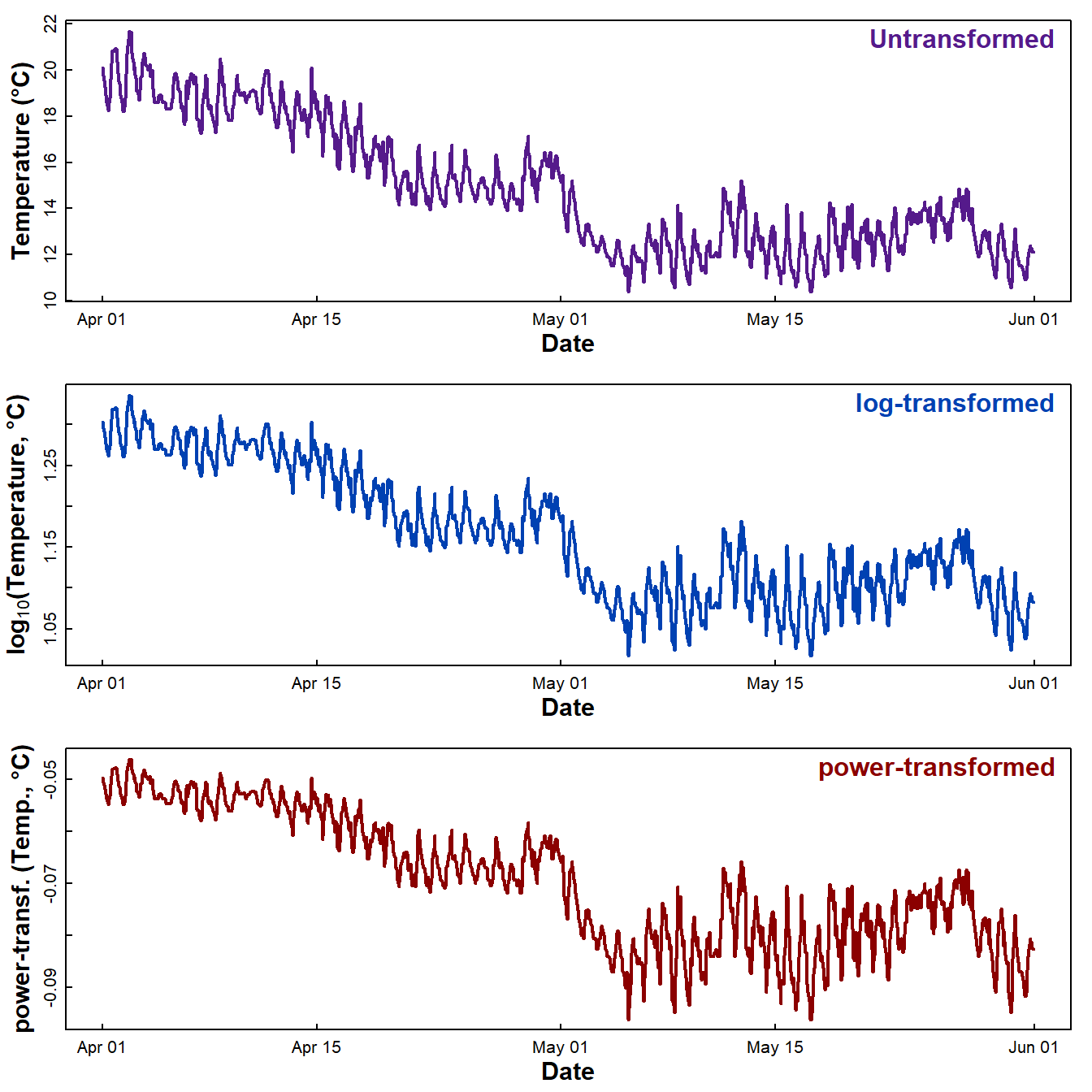
Figure 4: Plots of soil temperature time series data as untransformed, log₁₀-transformed, and power transformed values.
Which of these plots looks like it might be homoscedastic, i.e., have constant variance regardless of time?
The R Cookbook (Long and Teetor, 2019) suggests Box-Cox (power) transforming the variable to "stabilize the variance" (i.e. reduce heteroscedasticity). This does work, but can be better to use log10[variable], as the values are easier to interpret.
There are tests for homoscedasticity, usually based on the residuals from fitting a model (e.g. the Breusch-Pagan test). For our purposes visual assessment is enough.
If we think a transformation is needed, then run something like the
code below (which does a square root transformation, i.e.
variable0.5). This is just an example – we may, for example,
decide that the log10-transformation is more suitable. If we
save the results of powerTransform() to an object, it's
most convenient to use the rounded power term (e.g.
pt0$roundlam).
soiltemp_T15_zoo <- soiltemp_T15_zoo^0.5 #### don't run this chunk of code...
# don't forget the xts version either!
soiltemp_T15_xts <- as.xts(soiltemp_T15_zoo) # ...it's just an example 😊
Assessing if a time series variable is stationary
A stationary variable's mean and variance are not dependent on time. In other words, for a stationary series, the mean and variance at any time are representative of the whole series.
If there is a trend for the value of the variable to increase or decrease, or if there are periodic fluctuations, we don't have a stationary time series.
Many useful statistical analyses and models for time series models need a stationary time series as input, or a time series that can be made stationary with transformations or differencing.
Testing for stationarity
# we need the package 'tseries' for the Augmented Dickey–Fuller (adf) Test
d0 <- adf.test(soiltemp_T15_zoo); print(d0)
##
## Augmented Dickey-Fuller Test
##
## data: soiltemp_T15_zoo
## Dickey-Fuller = -3.9515, Lag order = 11, p-value = 0.01141
## alternative hypothesis: stationary##
## Augmented Dickey-Fuller Test
##
## data: diff(soiltemp_T15_zoo, 1)
## Dickey-Fuller = -16.143, Lag order = 11, p-value = 0.01
## alternative hypothesis: stationary##
## Augmented Dickey-Fuller Test
##
## data: diff(diff(soiltemp_T15_zoo, 1), 1)
## Dickey-Fuller = -17.204, Lag order = 11, p-value = 0.01
## alternative hypothesis: stationary
Plot differencing for stationarity
The plots in Figure 5 below show that constant mean and variance
(i.e. stationarity) is achieved after a single differencing
step. The adf.test p-value suggests that the
non-differenced series is already stationary, but the first sub-plot in
Figure 5 does not seem to support this.
par(mfrow = c(3,1), mar = c(0,4,0,1), oma = c(4,0,1,0), cex.lab = 1.4,
    mgp = c(2.5,0.7,0), font.lab = 2)
plot(soiltemp_T15_zoo, ylab = "Raw data, no differencing",
     xlab="", xaxt="n", col = 11)
lines(loess.smooth(index(soiltemp_T15_zoo),coredata(soiltemp_T15_zoo)),
      col = 5, lwd = 3)
abline(lm(coredata(soiltemp_T15_zoo) ~ index(soiltemp_T15_zoo)), col = 3)
legend("topright", legend = c("soiltemp_T15_Data", "Loess smoothing","Linear model"),
       cex = 1.8, col = c(11,5,3), lwd = c(1,3,1), bty = "n")
mtext(paste("adf.test p value =",signif(d0$p.value,3)),
      side = 1, line = -1.2, adj = 0.05)
plot(diff(soiltemp_T15_zoo,1),
     ylab = "First differencing",
     xlab="", xaxt="n", col = 11)
abline(h = 0, col = "grey", lty = 2)
lines(loess.smooth(index(diff(soiltemp_T15_zoo,1)),coredata(diff(soiltemp_T15_zoo,1))),
      col = 5, lwd = 3)
abline(lm(coredata(diff(soiltemp_T15_zoo,1)) ~
            index(diff(soiltemp_T15_zoo,1))), col = 3)
mtext(paste("adf.test p value =",signif(d1$p.value,3)),
      side = 1, line = -1.2, adj = 0.05)
plot(diff(diff(soiltemp_T15_zoo,1),1),
     ylab = "Second differencing",
     xlab="Date", col = 11)
mtext("Date",side = 1, line = 2.2, font = 2)
abline(h = 0, col = "grey", lty = 2)
lines(loess.smooth(index(diff(diff(soiltemp_T15_zoo,1),1)),
                   coredata(diff(diff(soiltemp_T15_zoo,1),1))),
      col = 5, lwd = 3)
abline(lm(coredata(diff(diff(soiltemp_T15_zoo,1))) ~
            index(diff(diff(soiltemp_T15_zoo,1)))), col = 3)
mtext(paste("adf.test p value =",signif(d2$p.value,3)),
      side = 1, line = -1.2, adj = 0.05)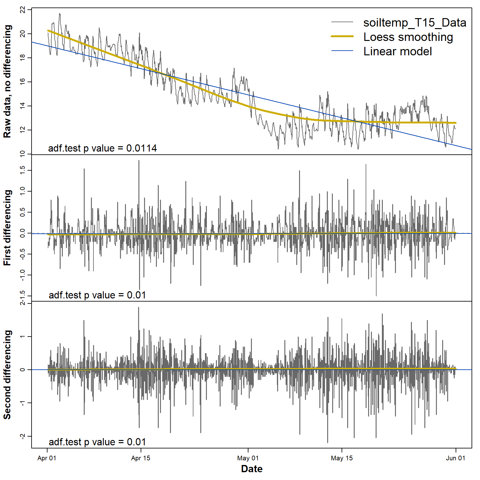
Figure 5: Plots of soil temperature time series data and its first and second differences, with each sub-plot showing the smoothed (Loess) and linear trends.
Finding the trend
A. Visualising a trend using a moving average
We create a new time series from a moving average for each 24h to
remove daily periodicity using the rollmean() function from
the zoo package. We know these are hourly data with diurnal
fluctuation, so a rolling mean for chunks of length 24 should be OK, and
this seems to be true based on Figure 6. In some cases the
findfrequency() function from the xts package
can detect the periodic frequency for us. A moving average will always
smooth our data, so a smooth curve doesn't necessarily mean that we have
periodicity (seasonality).
Moving averages are important parts of the ARIMA family of predictive models for time series, and that's why we show them here first.
There are possibly better ways of drawing smooth curves to represent our time series data... see below.
ff <- findfrequency(soiltemp_T15_xts) # often an approximation!! check the data!
cat("Estimated frequency is",ff,"\n")
## Estimated frequency is 24soiltemp_T15_movAv <- rollmean(soiltemp_T15_zoo, 24)
plot(soiltemp_T15_zoo, col=11, type="l") # original data
# add the moving average
lines(soiltemp_T15_movAv, lwd = 2, col=2)
legend("topright", bty="n", legend = c("Data","Moving average, \u0192 = 24"), col = c(8,2), lwd = c(1,2))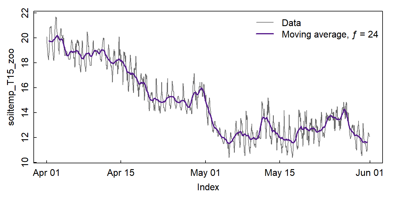
Figure 6: Plots of soil temperature time series data and the 24-hour moving average (ƒ = frequency).
B. Showing a trend using a linear (regression) model
This is just to visualize the trend. To find if a significant trend exists, we use the Mann-Kendall test or Sen's Slope test as described later.
First we create a linear model of the time series...
##
## Call:
## lm(formula = coredata(soiltemp_T15_zoo) ~ index(soiltemp_T15_zoo))
##
## Residuals:
##     Min      1Q  Median      3Q     Max
## -3.9217 -1.0968  0.0743  1.0938  3.5318
##
## Coefficients:
##                           Estimate Std. Error t value Pr(>|t|)
## (Intercept)              2.213e+03  3.370e+01   65.66   <2e-16 ***
## index(soiltemp_T15_zoo) -1.571e-06  2.409e-08  -65.22   <2e-16 ***
## ---
## Signif. codes:  0 '***' 0.001 '**' 0.01 '*' 0.05 '.' 0.1 ' ' 1
##
## Residual standard error: 1.402 on 1462 degrees of freedom
## Multiple R-squared:  0.7442, Adjusted R-squared:  0.744
## F-statistic:  4253 on 1 and 1462 DF,  p-value: < 2.2e-16
...then use a plot (Figure 7) to look at the linear relationship.
soiltemp_T15_lmfit <- zoo(lm0$fitted.values, index(soiltemp_T15_zoo))
plot(soiltemp_T15_zoo, col = 11, type = "l")
lines(soiltemp_T15_lmfit, col = 2, lty = 2, lwd=2)
legend("topright", bty="n", legend = c("Data","Linear trend"), col = c(8,2), lty = c(1,2), lwd=c(1,2), seg.len=3)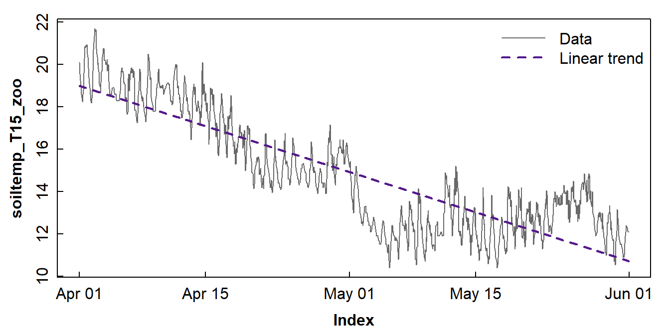
Figure 7: Plots of soil temperature time series data and the overall trend shown by a linear model.
Figure 7 shows that a linear model does not really capture the trend (even without considering the periodicity) very convincingly. The next option, 'loess' smoothing, shown below tries to represent the trend more accurately.
C. Using Locally Estimated Scatterplot Smoothing (loess)
loess, sometimes called 'lowess' is a form of
locally weighted non-parametric regression to fit smooth curves to data.
The amount of smoothing is controlled by the span =
parameter in the loess.smooth() function (from base
R) – see the example using the soil temperature data in
Figure 8.
y_trend <- loess.smooth(index(soiltemp_T15_zoo),
                           coredata(soiltemp_T15_zoo),
                           span = 0.15, evaluation = length(soiltemp_T15_zoo))
plot(soiltemp_T15_zoo, col = 11, type = "l")
soiltemp_T15_trend <- zoo(y_trend$y, index(soiltemp_T15_zoo))
lines(soiltemp_T15_lmfit, col = 2, lty = 2)
lines(soiltemp_T15_trend, col = 4, lwd = 3)
legend("topright", bty = "n", inset = 0.02, cex = 1.25,
       legend = c("actual data","linear model","loess smoothed"),
       col = c(11,2,4), lty=c(1,2,1), lwd = c(1,1,3))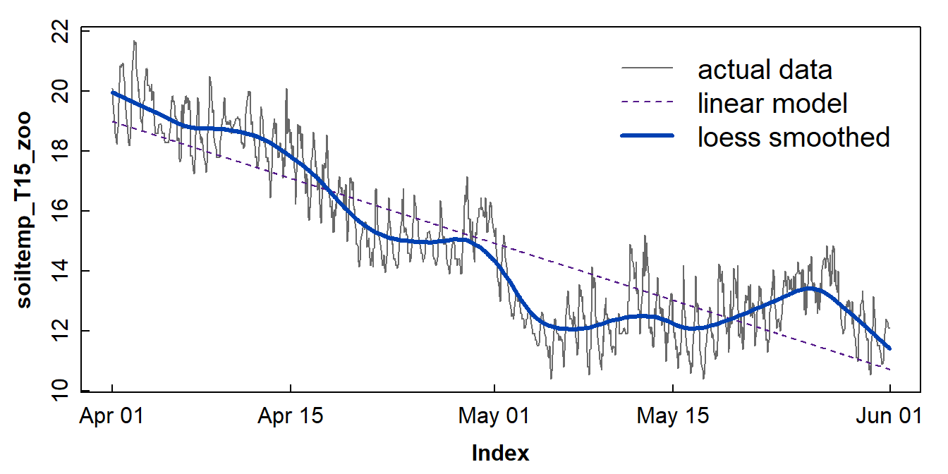
Figure 8: Plots of soil temperature time series data and the overall trend shown by a loess smoothing model.
Isolating the Time Series Periodicity
NOTE THAT TIME SERIES DON'T ALWAYS HAVE PERIODICITY !
To model the periodicity it is useful to understand the
autocorrelation structure of the time series. We can do this
graphically, first by plotting the autocorrelation function
acf() which outputs a plot by default:
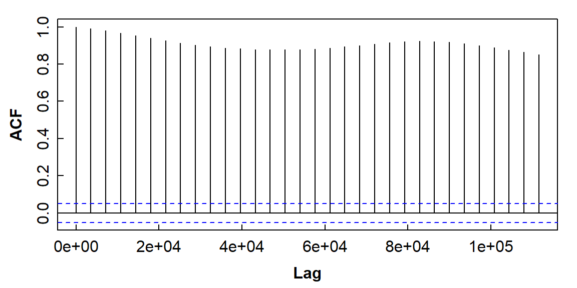
Figure 9: The autocorrelation function plot for soil temperature time series data (the horizontal axis is in units of seconds).
What does Figure 9 tell you about autocorrelation in this time series?
Then plot the partial autocorrelation function
(pacf())
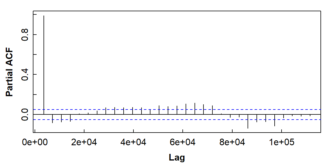
Figure 10: The partial autocorrelation function plot for soil temperature time series data (horizontal axis units are seconds).
Interpreting partial autocorrelations (Figure 10) is more complicated – refer to Long & Teetor (2019, Section 14.15). Simplistically, partial autocorrelation allows us to identify which and how many autocorrelations will be needed to model the time series data.
Box-Pierce test for autocorrelation
The null hypothesis H0 for the Box-Pierce test
(Box.test())is that no autocorrelation exists at any lag
distance (so p ≤ 0.05 'rejects' H0):
##
##  Box-Pierce test
##
## data:  soiltemp_T15_xts
## X-squared = 1436.3, df = 1, p-value < 2.2e-16##
## Box-Pierce test
##
## data: diff(soiltemp_T15_xts, 1)
## X-squared = 15.658, df = 1, p-value = 7.589e-05##
## Box-Pierce test
##
## data: diff(diff(soiltemp_T15_xts, 1), 1)
## X-squared = 357.45, df = 1, p-value < 2.2e-16
Make a time series of the loess residuals
Remember that we made a loess model of the time series
... the residuals (Figure 11) can give us the combination of periodicity
component plus any random variation.
soiltemp_T15_periodic <- soiltemp_T15_zoo - soiltemp_T15_trend
plot(soiltemp_T15_trend, ylim = c(-2,20), lty = 3)
lines(soiltemp_T15_periodic, col = 6, lwd = 2) # just to check
legend("topright", legend = c("LOESS trend", "Periodicity plus noise"),
       col = c(1,6), lwd = c(1,2), lty = c(3,1))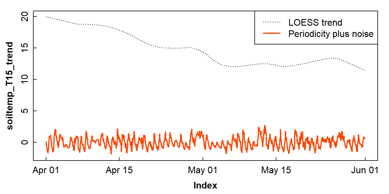
Figure 11: An incomplete decomposition of the soil temperature time series into smoothed trend and periodicity plus error (noise) components.
We can also use less smoothing in the loess function to
retain periodicity; we adjust the span = option
(lower values of span give less smoothing; we just need to
experiment with different values). The difference between the data and
the less-smoothed loess should be just 'noise' or
'error'.
We first generate a loess model which is stored in the object
temp_LOESS2:
temp_LOESS2 <- loess.smooth(index(soiltemp_T15_zoo),
                           coredata(soiltemp_T15_zoo),
                           span = 0.012, evaluation = length(soiltemp_T15_zoo))
We then use the new loess model to make a time series which contains both periodic and trend information:
The difference between the data and the less-smoothed loess should be just 'noise' or 'error', so we make a new time series based on this difference:
Then plot, setting y axis limits to similar scale to original data:
plot(soiltemp_T15_trend, ylim = c(-2,20), lty = 2, lwd = 2, # from above
     xlab = "2014 Date", ylab = "Soil temperature (\u00B0C)")
lines(soiltemp_T15_LOESS2, col = 3, lwd = 2)
lines(soiltemp_T15_err, col = 5) # from a couple of lines above
legend("left",
       legend = c("Trend (coarse LOESS)",
                  "Periodicity + trend (fine LOESS)",
                  "Unexplained variation"),
       col = c(1,3,5), lwd = c(2,2,1), lty = c(2,1,1), bty="n")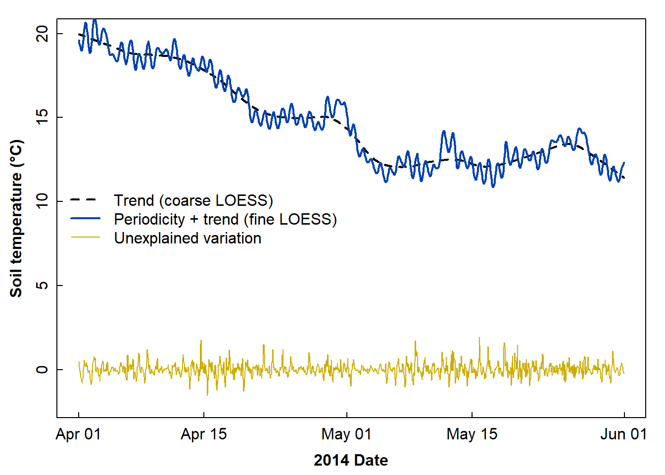
Figure 12: Incomplete decomposition of soil temperature time series data showing the smoothed trend, combined trend + periodicity, and error components.
We're now in a position to estimate homoscedasticity of our time
series. It's a bit ‘hacky’, but we can predict the raw time series from
the smoothed trend+periodicity, then apply the Breusch-Pagan test to our
model (we need the lmtest package loaded earlier for the
bptest() function):
##
##  studentized Breusch-Pagan test
##
## data:  lm0
## BP = 0.087412, df = 1, p-value = 0.7675
The bptest() p-value is > 0.05 so, by this estimate,
our time series is homoscedastic.
The periodicity by itself should be represented by the difference between the very smoothed (trend) and less smoothed (trend + periodicity) loess, as suggested by the two loess curves in Figure 12. We now make yet another time series object to hold this isolated periodicity:
Show the components of time series decomposition
plot(cbind(soiltemp_T15_zoo,soiltemp_T15_periodic2,
     soiltemp_T15_trend, soiltemp_T15_err), main = "",
     xlab = "Date in 2014",
     cex.main = 1.5, yax.flip = TRUE, col = c(2,3,4,5),
     ylim = c(floor(min(soiltemp_T15_periodic2)),
              ceiling(max(soiltemp_T15_zoo))))
x1 <- (0.5*(par("usr")[2]-par("usr")[1]))+par("usr")[1]
y <- (c(0.18, 0.3, 0.6, 0.82)*(par("usr")[4]-par("usr")[3]))+par("usr")[3]
text(rep(x1,4), y,
     labels = c("Unaccounted variation","Trend","Apparent periodicity","Data"),
     col = c(5,4,3,2))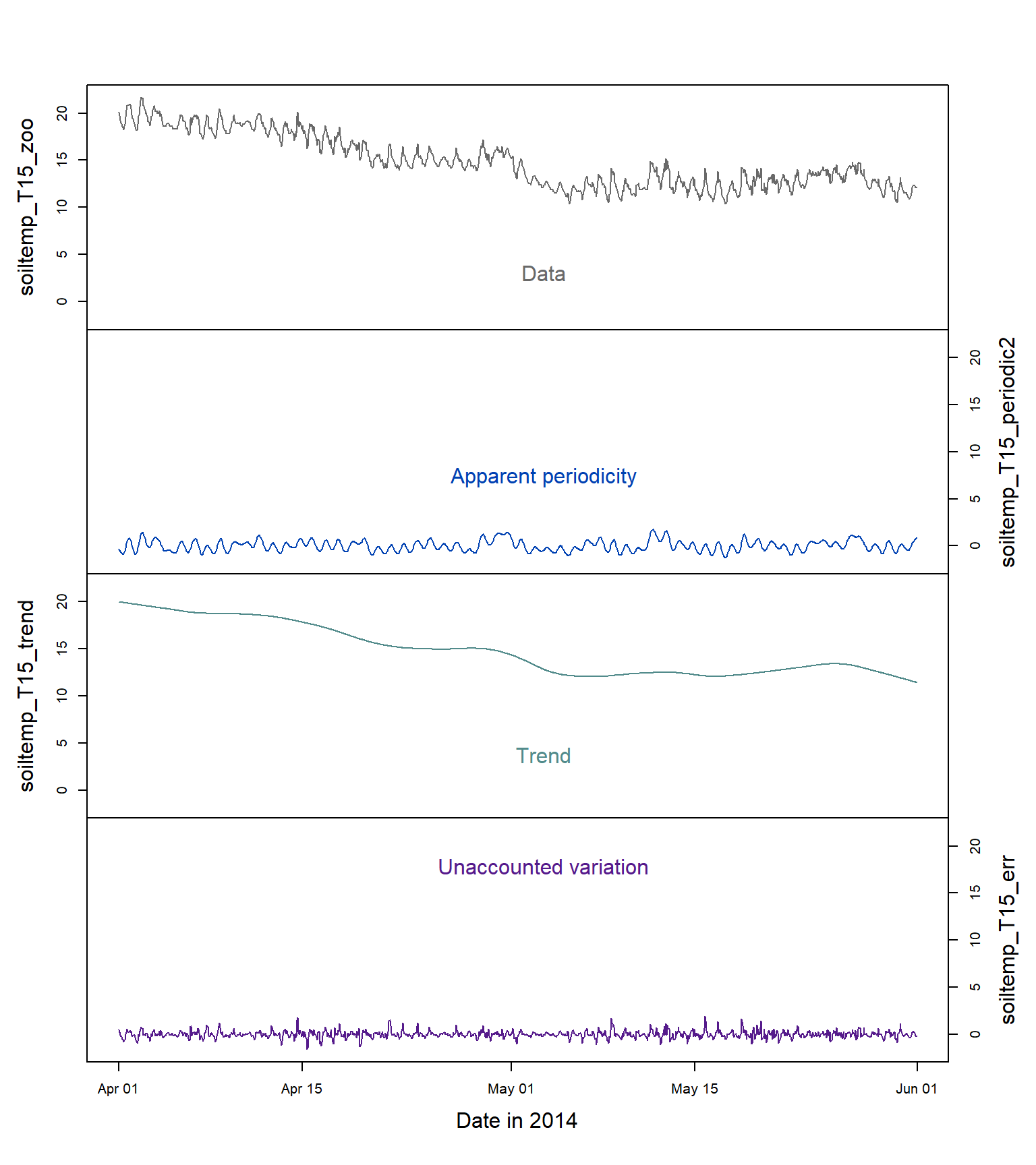
Figure 13: Time series decomposition into the three main components (periodicity, trend, and error; the raw data are at the top) for soil temperature (°C) at 15 cm depth.
Figure 13 shows the original time series data, and the three important components of the decomposed time series: the periodicity, the trend, and the error or unexplained variation. We should remember that:
- this time series was relatively easy to decompose into its components, but not all time series will be so 'well-behaved';
- there are different ways in which we can describe the trend and periodicity (we have just used the loess smoothing functions for clear visualization).
This ends
our exploratory data analysis of time series, which leads us into time
series models,
including trend and ARIMA forecast
modelling.
3. Models for Time Series – Trends and Forecasts
Trends and forecasts of time series are the types of analyses we would typically report on (see box below).
Trends in time series
The simplest model for time series is a trend, i.e. an overall increase or decrease. We don't use the usual correlation or regression statistics, as we expect autocorrelation in a time series, so the observations are not independent. We need to use statistical tests that can handle the autocorrelation dependence between observations, and these are described below.
(a) Apply the Mann-Kendall test from the 'trend' package
##
##  Mann-Kendall trend test
##
## data:  coredata(soiltemp_T15_zoo)
## z = -36.387, n = 1464, p-value < 2.2e-16
## alternative hypothesis: true S is not equal to 0
## sample estimates:
##             S          varS           tau
## -6.797270e+05 3.489630e+08 -6.371125e-01The output from mk.test() shows a negative slope
(i.e. the value of S), with the
p-value definitely < 0.05, so we can reject the null
hypothesis of zero slope.
(b) Estimate the Sen's slope
##
##  Sen's slope
##
## data:  coredata(soiltemp_T15_zoo)
## z = -36.387, n = 1464, p-value < 2.2e-16
## alternative hypothesis: true z is not equal to 0
## 95 percent confidence interval:
##  -0.005963303 -0.005570410
## sample estimates:
##  Sen's slope
## -0.005765595
The output from sens.slope() also shows a negative slope
(i.e. the value of Sen's slope at the end of the
output block). Again, the p-value is < 0.05, so we can
reject the null hypothesis of zero slope. The
95 percent confidence interval does not include zero, also
showing that the Sen's slope is significantly negative in this
example.
Modelling time series with ARIMA
All the analysis of our data before ARIMA is really exploratory data analysis of time series:
- Does our time series have periodicity (seasonality)?
- Can we get the trend with a moving average?
- Does our time series have autocorrelation?
- Can we get stationarity by differencing?
All of these properties are possible components of ARIMA models!
We recommend using the xts
format of a time series in ARIMA model functions and
forecasting.
Use the forecast R package to create an ARIMA
model
## Series: soiltemp_T15_xts
## ARIMA(1,0,3) with non-zero mean
##
## Coefficients:
##          ar1     ma1     ma2     ma3     mean
##       0.9883  0.0923  0.0892  0.0999  15.0050
## s.e.  0.0041  0.0263  0.0255  0.0258   0.9301
##
## sigma^2 = 0.1188:  log likelihood = -517.87
## AIC=1047.73   AICc=1047.79   BIC=1079.47
The auto.arima() function runs a complex algorithm
(Hyndman et al. 2020) to automatically select the best ARIMA
model on the basis of the Aikake Information Criterion
(AIC), a statistic which estimates how much information is 'lost' in the
model compared with reality. The AIC combines how well the model
describes the data with a 'penalty' for increased complexity of the
model. Using AIC, a better fitting model might not be selected if it has
too many predictors. The best ARIMA models will have the
lowest AIC (or AICc) value.
Use output of auto.arima() to run arima
The auto-arima() algorithm is not perfect! – but it does
provide a starting point for examining ARIMA models. The output of the
auto-arima() function includes a description of the best
model the algorithm found, shown as ARIMA(p,d,q). The
p,d,q are defined in Table 1
below:
Parameter | Meaning | Informed by |
|---|---|---|
p | The number of autoregressive predictors | Partial autocorrelation |
d | The number of differencing steps | Stationarity tests ± differencing |
q | The number of moving average predictors | Stationarity tests ± moving averages |
A periodic or seasonal ARIMA model (often called SARIMA) has
a more complex specification:
ARIMA(p,d,q)(P,D,Q)(n) ,
where the additional parameters refer to the seasonality:
P is the number of seasonal autoregressive predictors,
D the seasonal differencing, Q the seasonal
moving averages, and n is the number of time steps per
period/season.
(a) With no seasonality
##
## Call:
## arima(x = soiltemp_T15_xts, order = c(1, 0, 3))
##
## Coefficients:
##          ar1     ma1     ma2     ma3  intercept
##       0.9883  0.0923  0.0892  0.0999    15.0050
## s.e.  0.0041  0.0263  0.0255  0.0258     0.9301
##
## sigma^2 estimated as 0.1184:  log likelihood = -517.87,  aic = 1047.73
##
## Training set error measures:
##                        ME      RMSE       MAE         MPE     MAPE     MASE
## Training set -0.005215705 0.3441525 0.2467179 -0.08670514 1.716531 0.980305
##                       ACF1
## Training set -0.0001019764
##                 2.5 %     97.5 %
## ar1        0.98017359  0.9963265
## ma1        0.04074353  0.1438382
## ma2        0.03916128  0.1392272
## ma3        0.04923344  0.1504821
## intercept 13.18199812 16.8279311
The output from summary(am0) shows the values and
uncertainties of the model parameters
(ar1, ma1, ma2, ma3, intercept), the goodness-of-fit
parameters (we're interested in aic).
Note: ar parameters are auto-regression
coefficients, and ma are moving average coefficients.
The output from confint(am0) is a table showing the 95%
confidence interval for the parameters. The confidence intervals should
not include zero! (if so, this would mean we can't be sure if the
parameter is useful or not).
(b) With seasonality
ff <- findfrequency(soiltemp_T15_xts)
cat("Estimated time series frequency is",ff,"\n")
am1 <- arima(x = soiltemp_T15_xts, order = c(1,0,2),
             seasonal = list(order = c(1, 0, 1), period = ff))
summary(am1)
confint(am1)
## Estimated time series frequency is 24
##
## Call:
## arima(x = soiltemp_T15_xts, order = c(1, 0, 2), seasonal = list(order = c(1,
## 0, 1), period = ff))
##
## Coefficients:
## ar1 ma1 ma2 sar1 sma1 intercept
## 0.9968 -0.1466 -0.0984 0.9998 -0.9856 14.829
## s.e. 0.0020 0.0268 0.0288 0.0004 0.0143 10.415
##
## sigma^2 estimated as 0.09073: log likelihood = -355.68, aic = 725.35
##
## Training set error measures:
## ME RMSE MAE MPE MAPE MASE
## Training set -0.01572894 0.30122 0.2169846 -0.1427709 1.504911 0.8621632
## ACF1
## Training set 0.0006582706
## 2.5 % 97.5 %
## ar1 0.9928401 1.00080710
## ma1 -0.1990623 -0.09412079
## ma2 -0.1549117 -0.04197365
## sar1 0.9989639 1.00061967
## sma1 -1.0136981 -0.95746903
## intercept -5.5840446 35.24194848Note: sar parameters are seasonal
auto-regression coefficients, and sma are seasonal
moving average coefficients.
The model which includes periodicity has the lowest AIC value (which is not surprising, since the soil temperature data have clear periodicity).
Checking residuals using the checkresiduals() function
from the forecast package is our best diagnostic tool to
assess the validity of our models. [This is a separate issue from how
well the model describes the data, measured by AIC. Also, we can't use
bptest() to analyse ARIMA residuals.]
In the output (plot and text) from checkresiduals(): -
the residual plot (top) should look like white noise - the residuals
should not be autocorrelated (bottom left plot) - the p-value from the
Ljung-Box test should be > 0.05 (text output) - the residuals should
be normally distributed (bottom right plot)
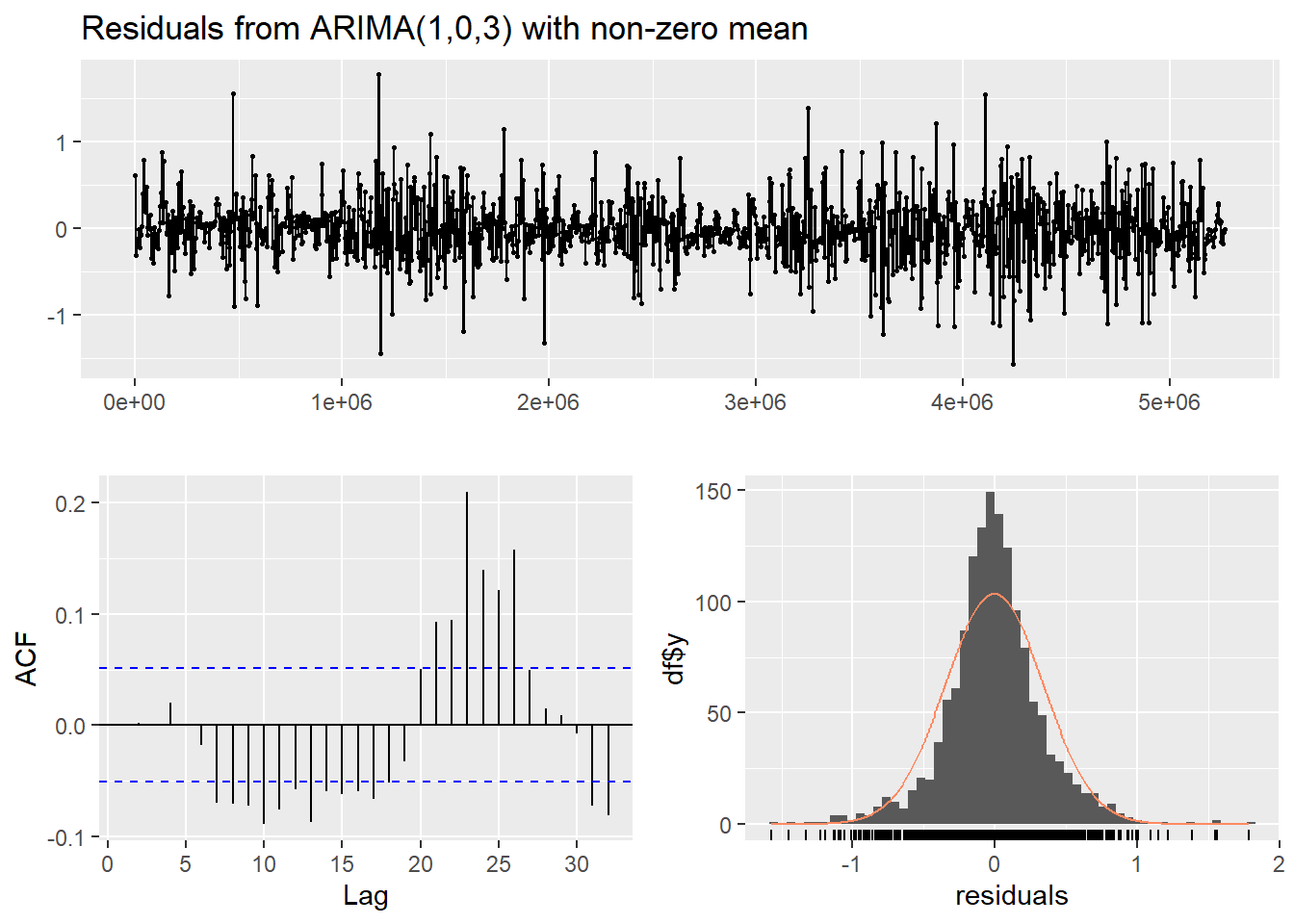
Figure 14: Residual diagnostic plots for a non-seasonal ARIMA model of the soil temperature time series.
##
##  Ljung-Box test
##
## data:  Residuals from ARIMA(1,0,3) with non-zero mean
## Q* = 35.092, df = 6, p-value = 4.136e-06
##
## Model df: 4.   Total lags used: 10
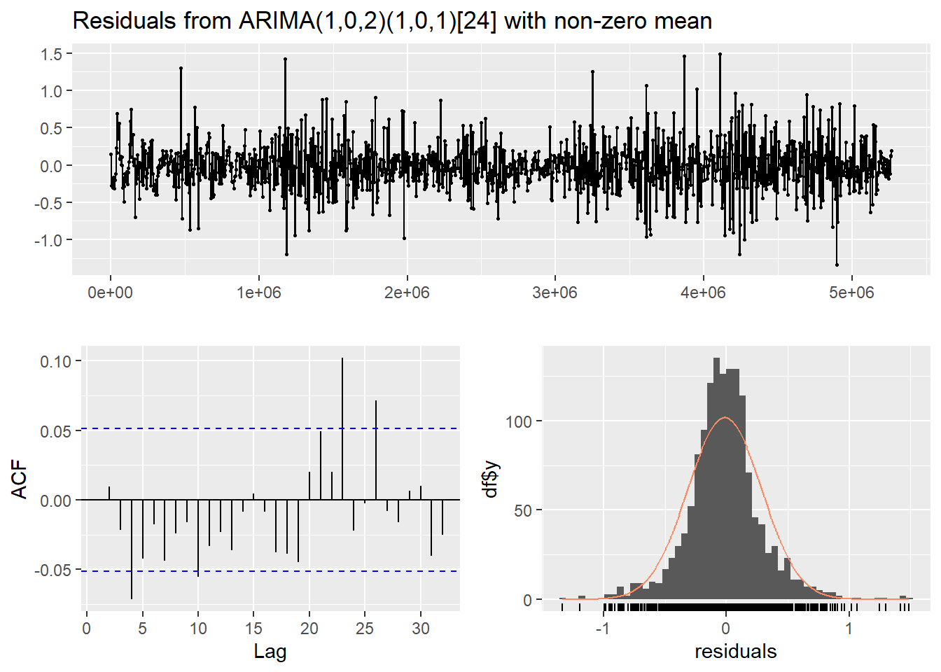
Figure 15: Residual diagnostic plots for a seasonal ARIMA (SARIMA) model of the soil temperature time series.
##
##  Ljung-Box test
##
## data:  Residuals from ARIMA(1,0,2)(1,0,1)[24] with non-zero mean
## Q* = 20.04, df = 5, p-value = 0.001228
##
## Model df: 5.   Total lags used: 10
In both the diagnostic plots (Figure 14 and Figure 15) the residuals appear to be random and normally distributed. There seems to be a more obvious autocorrelation of residuals for the non-seasonal model, reinforcing the conclusion from the AIC value that the seasonal ARIMA model is the most appropriate.
Looking at how well (or not) the (S)ARIMA models fit the actual data
In Figure 16 (below) we can see how well the ARIMA and seasonal ARIMA
models fit the data (for clarity, only one week of hourly observations
are plotted, otherwise there is a lot of overlap). The ARIMA objects
am0 and am1 don't contain the fitted values,
but they do contain model residuals so we calculate
fitted = observed - residual in each case.
Note that a non-seasonal ARIMA model can still capture periodicity by making predictions based just on autocorrelation and moving averages. The fit of both the ARIMA and SARIMA models to the actual data seems similar based on these plots; we see how the models differ below, when we try to use the models for forecasting.
rz <- c(721:888) # vector of row numbers to represent 1 week (168 hours)
par(mar=c(3,3.5,0.5,0.5), mgp=c(1.6,0.3,0), tcl=0.2, font.lab=2, cex.lab=1.4,
    cex.axis=1.2, lend="square", mfrow=c(2,1))
palette(c("black", plasma(4, end=0.5),plasma(4, alpha=0.5, begin=0.5),"white"))

plot(soiltemp_T15_zoo[rz,], type="n", lwd=1, xlab="Date", ylab="Soil temperature (\u00b0C)")
lines(index(soiltemp_T15_zoo[rz,]), coredata(soiltemp_T15_zoo[rz,])-am0$residuals[rz],
      col=6, lwd=5)
points(soiltemp_T15_zoo[rz,], type="p", col=2, pch=3)
mtext("(a)",3,-1.5, adj=0.98, cex=1.4)
legend("bottomleft", box.col="grey", legend=c("Observed data","ARIMA model"),
       pch=c(3,NA), lwd=c(NA,3), lty=c(NA,1),
       col=c(2,6), inset=0.02, cex=1.4)

plot(soiltemp_T15_zoo[rz,], type="n", lwd=1, xlab="Date",
     ylab="Soil temperature (\u00b0C)")
lines(index(soiltemp_T15_zoo[rz,]), coredata(soiltemp_T15_zoo[rz,])-am1$residuals[rz],
      col=7, lwd=5)
points(soiltemp_T15_zoo[rz,], type="p", col=2, pch=3)
legend("bottomleft", box.col="grey", legend=c("Observed data", "Seasonal ARIMA model"),
       pch=c(3,NA), lwd=c(NA,3), lty=c(NA,1), col=c(2,7), inset=0.02, cex=1.4)
mtext("(b)",3,-1.5, adj=0.98, cex=1.4)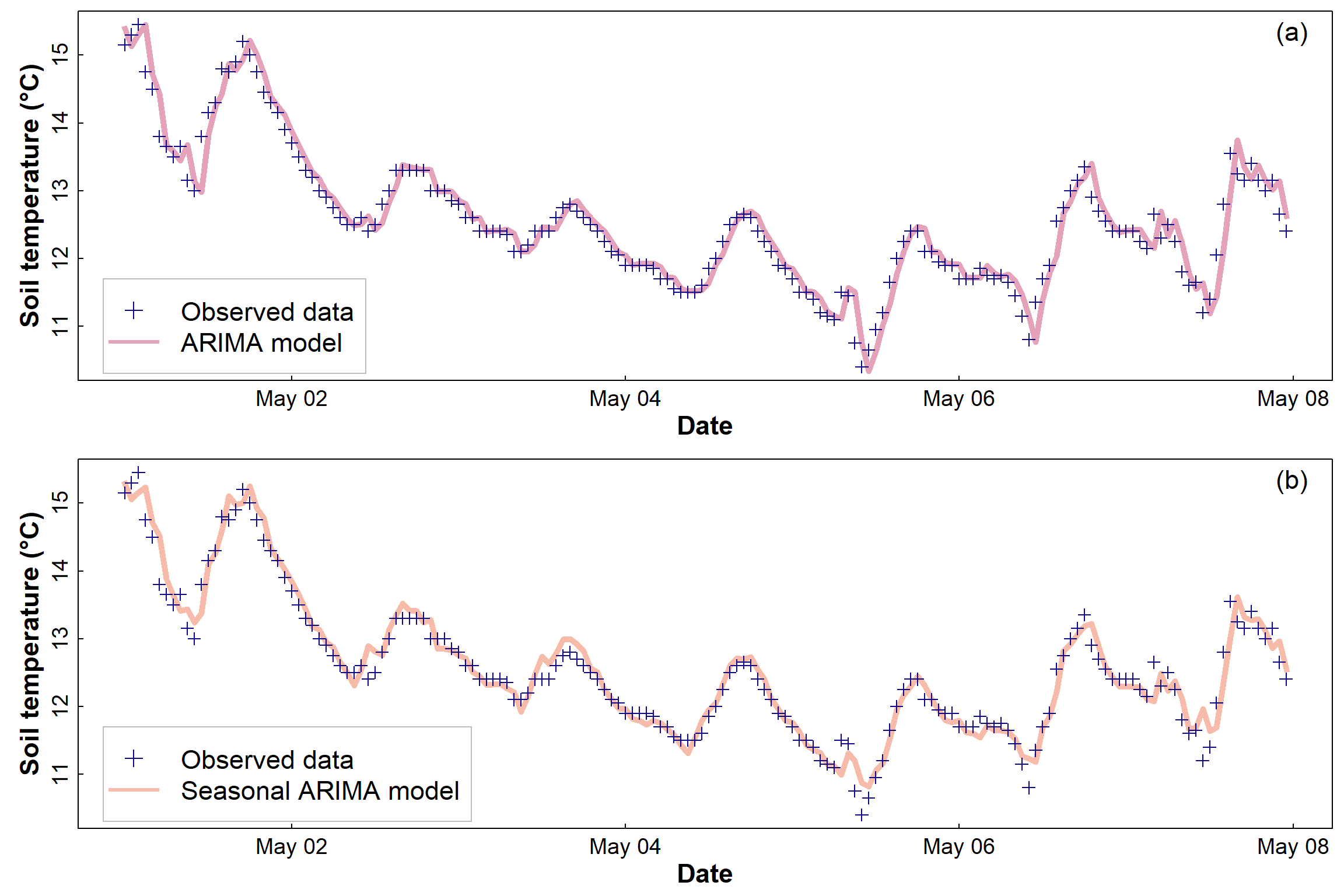
Figure 16: Soil temperature data for the first week of May 2014, showing (a) the fitted ARIMA model and (b) the fitted SARIMA (seasonal) model. The thickness of the fitted lines in both (a) and (b) is arbitrary and does not represent model uncertainty.
Use the ARIMA model to produce a forecast using both models
The whole point of generating ARIMA models is so that we can attempt to forecast the future trajectory of our time series based on our existing time series data.
To do this, we use the appropriately named forecast()
function from the forecast package. The option
h = is to specify how long we want to forecast for after
the end of our data – in this case 168 hours (same units as the
periodicity from findfrequency()), that is, one week.
One of the problems we often run into is the issue of irregular time series, where the observations are not taken at regularly-spaced time intervals. Features of time series, such as periodicity and the length of time we want to forecast for, may be incorrect if our time series is irregular.
It is possible to "fill in" a time series so we have observations regularly spaced in time, using interpolation or numerical filtering methods. We won't be covering these methods here, though.
Then, look at forecasts with plots
par(mfrow = c(2, 1), cex.main = 0.9, mar = c(0,3,0,1), oma = c(3,0,1,0),
    mgp=c(1.6,0.3,0), tcl=0.2, font.lab=2)
plot(fc0,ylab = "Temperature (\u00B0C)",
     fcol = 7, xlab="", main = "", xaxt="n")
lines(soiltemp_T15_zoo, col = "grey70")
mtext("ARIMA with no seasonality", 1, -2.2, adj = 0.1, font = 2)
mtext(am0$call, 1, -1, adj = 0.1, col = 7, cex = 0.9,
      family="mono", font = 2)
mtext("(a)", 3, -1.2, cex = 1.2, font = 2, adj = 0.95)

plot(fc1,ylab = "Temperature (\u00B0C)", main = "", fcol = 3)
lines(soiltemp$conc, col = "grey70")
mtext("Time since start (seconds)", 1, 1.7, cex = 1.2, font = 2)
mtext(paste("ARIMA with",am1$arma[5],"h periodicity"),
      side = 1, line = -2.2, adj = 0.1, font = 2)
mtext(am1$call, 1, -1, adj = 0.1, col = 3, cex = 0.9, family="mono")
mtext("(b)", 3, -1.2, cex = 1.2, font = 2, adj = 0.95)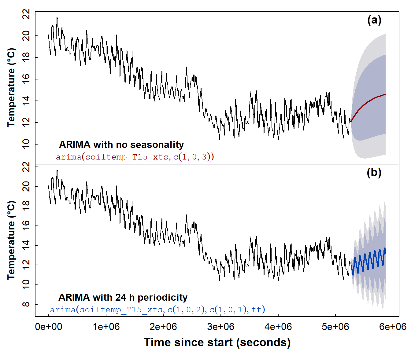
Figure 17: Time series forecasts for soil temperature, based on (a) a non-seasonal ARIMA model and (b) a seasonal ARIMA model.
From the two plots in Figure 17, we observe that the seasonal ARIMA model seems to reflect the form of the original data much better, by simulating the diurnal fluctuations in soil temperature. Although the forecasting uncertainty shown by the shaded area in Figure 17 is large for both types of ARIMA model, the interval seems smaller for the seasonal ARIMA model (Figure 17(b)).
We can also make a slightly 'prettier' time series forecast plot
using the autoplot() function from the ggplot2
package (Figure 18):
require(ggplot2) # gives best results using autoplot(...)
autoplot(fc1)+
  ylab("Temperature (\u00B0C)") +
  xlab(paste("Time since",index(soiltemp_T15_zoo)[1],"(s)")) +
  ggtitle("") +
  theme_bw()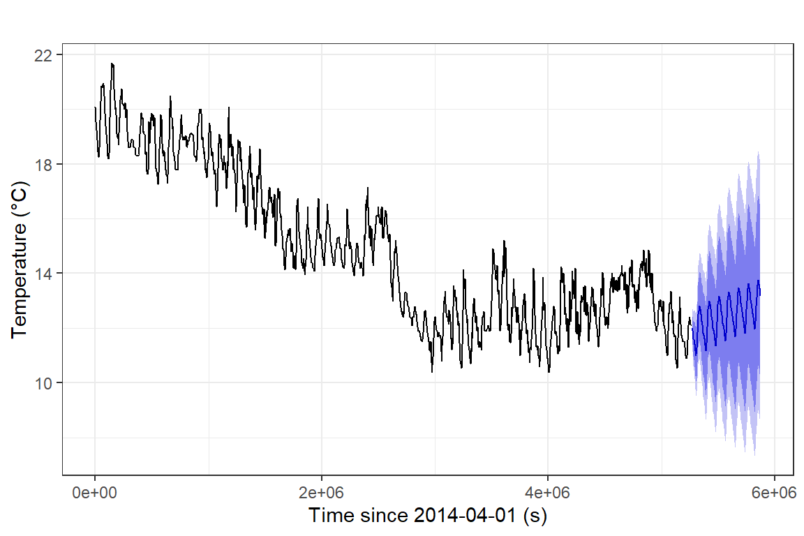
Figure 18: Time series forecast for soil temperature, based on a
seasonal ARIMA model, plotted using the ggplot2 autoplot()
function.
ARIMA models are not the end of the time series modelling and forecasting story!
Exponential Smoothing Models
Sometimes, ARIMA models may not be the best option, and another commonly used method is exponential smoothing.
Check help(forecast::ets) to correctly specify the model
type using the model = option!
The easiest option (and the one used here) is to specify
model = "ZZZ", which chooses the type of model
automatically.
## Warning in ets(soiltemp_T15_xts, model = "ZZZ"): Non-integer seasonal period.
## Only non-seasonal models will be considered.## ETS(A,Ad,N)
##
## Call:
## ets(y = soiltemp_T15_xts, model = "ZZZ")
##
## Smoothing parameters:
## alpha = 0.9999
## beta = 0.1083
## phi = 0.8
##
## Initial states:
## l = 20.2683
## b = -0.4487
##
## sigma: 0.3482
##
## AIC AICc BIC
## 7588.660 7588.718 7620.394
##
## Training set error measures:
## ME RMSE MAE MPE MAPE MASE
## Training set -0.003041526 0.3475639 0.2472475 -0.03856289 1.719534 0.01664266
## ACF1
## Training set 0.0146761In this case the ets() function has automatically
selected a model (ETS(A,Ad,N)) with additive trend and
errors, but no seasonality. We don't do it here, but we could manually
select a model with seasonality included.
The default plot function in R can plot forecasts from exponential smoothing models too (Figure 19).
plot(forecast(soiltemp_T15_ets, h=168), col=2, fcol=5,
     xlab = "Time since start (s)", ylab = "Temperature (\u00B0C)", main="")
mtext(names(soiltemp_T15_ets$par),3,seq(-1,-5,-1), adj = 0.7, col = 5, font = 3)
mtext(signif(soiltemp_T15_ets$par,3),3,seq(-1,-5,-1), adj = 0.8, col = 5, font = 3)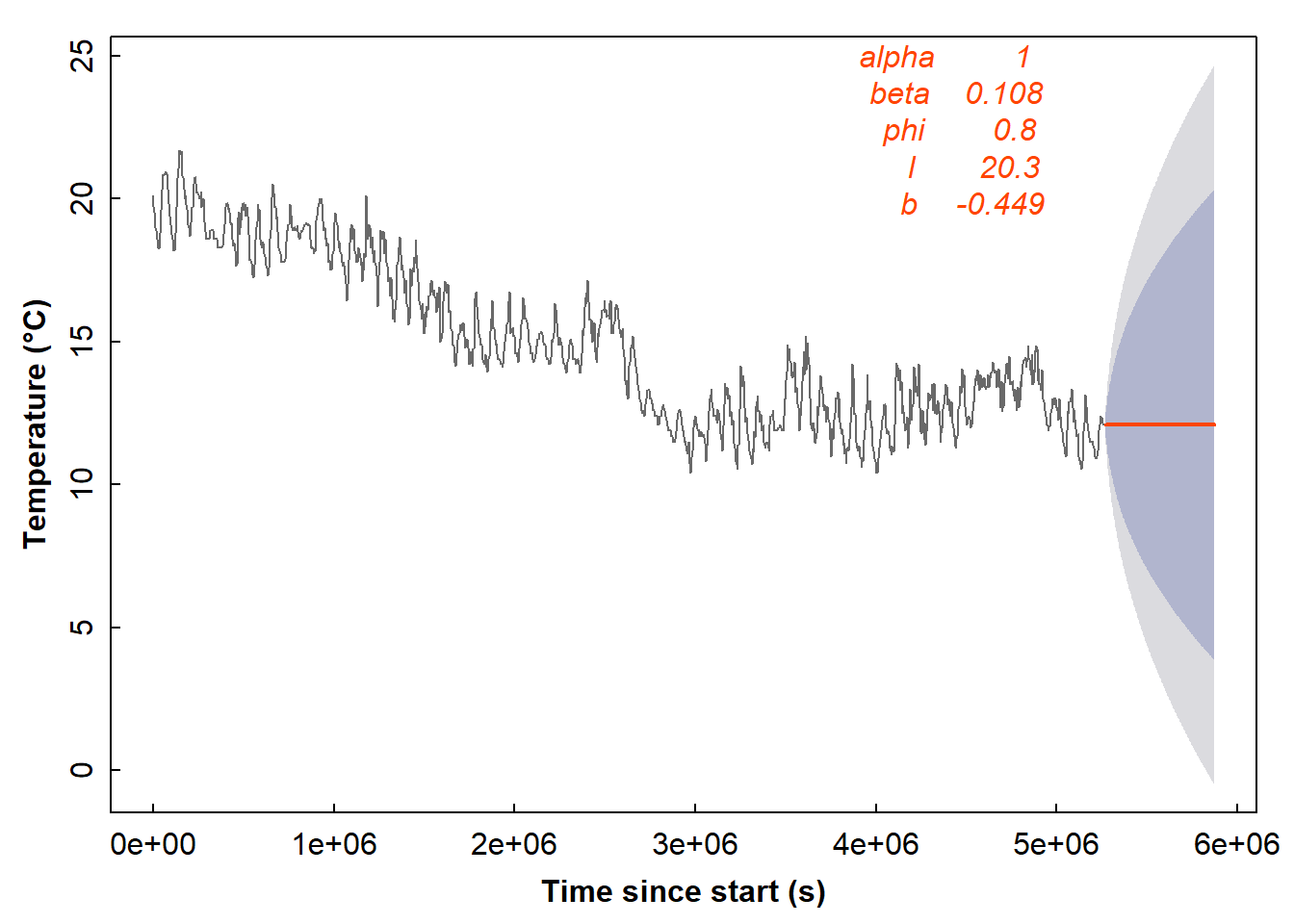
Figure 19: Forecast of soil temperature based on an automatically selected exponential smoothing model without a seasonal component.
Exponential smoothing also decomposes time series in a different way, into level and slope components (Figure 20).
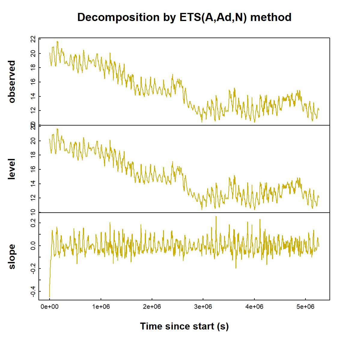
Figure 20: Exponential smoothing time series decomposition plots for soil temperature data.
(Exponential smoothing is maybe not so good for the soil temperature data!)
References
Australian Government (2023). Assessment of change through monitoring data analysis, In Australian & New Zealand Guidelines for Fresh and Marine Water Quality, www.waterquality.gov.au/anz-guidelines/monitoring/data-analysis/data-assess-change.
Department of Water (2015). Calculating trends in nutrient data, Government of Western Australia, Perth. www.wa.gov.au/.../calculating-trends-nutrient-data.
Hyndman R, Athanasopoulos G, Bergmeir C, Caceres G, Chhay L,
O'Hara-Wild M, Petropoulos F, Razbash S, Wang E, Yasmeen F (2022).
forecast: Forecasting functions for time
series and linear models. R package version 8.17.0, http://pkg.robjhyndman.com/forecast/.
Long, J.D., Teetor, P., 2019. Time series analysis. Chapter 14, The R Cookbook, Second Edition https://rc2e.com/timeseriesanalysis.
R Core Team (2022). R: A language and environment
for statistical computing. R Foundation for Statistical Computing,
Vienna, Austria. URL https://www.R-project.org/.
Ryan, J.A. and Ulrich, J.M. (2020). xts: eXtensible
Time Series. R package version 0.12.1. https://CRAN.R-project.org/package=xts
Smith, A. B., Walker, J. P., Western, A. W., Young, R. I., Ellett, K. M., Pipunic, R. C., Grayson, R. B., Siriwidena, L., Chiew, F. H. S. and Richter, H. (2012) The Murrumbidgee Soil Moisture Monitoring Network Data Set. Water Resources Research, 48:W07701 doi:10.1029/2012WR011976
Zeileis, A. and Grothendieck, G. (2005). zoo: S3
Infrastructure for Regular and Irregular Time Series. Journal of
Statistical Software, 14(6), 1-27. doi:10.18637/jss.v014.i06
CC-BY-SA • All content by Ratey-AtUWA. My employer does not necessarily know about or endorse the content of this website.
Created with rmarkdown in RStudio. Currently using the free yeti theme from Bootswatch.