 Material to support teaching in Environmental Science at The University of Western Australia
Units ENVT3361, ENVT4461, and ENVT5503
R markdown chunk options
More control over reports
Andrew Rate
2025-12-04
This brief guide follows on from a previous page on this site, the Brief Essentials of R Markdown
Hiding both code and output
 If we want R code to run, but not show either the code
nor any output, we include the option
If we want R code to run, but not show either the code
nor any output, we include the option include=FALSE. We
might do this if it's not important for readers to see the code, for
example setting overall document options. For UWA assignments, it's
usually essential to show which R packages you used, so don't hide the
code which loads these!
# the R markdown chunk option include = FALSE is used when it's not
# helpful to see the code and output, for example setting options
knitr::opts_chunk$set(echo = FALSE, warning = FALSE, message = FALSE)
set_flextable_defaults(theme_fun = "theme_zebra", font.size = 10, fonts_ignore = TRUE)
```
☝ this code would not appear in the knitted document since
include=FALSE ☝
Chunk Names: You'll notice that after
{r we include a name like
hide-code-and-output. These names must be unique for each
chunk, preferably with words separated with hyphens -.
Usually we don't want warnings or messages from our R
code in reports either, so we would also include
warning=FALSE and include=FALSE:
⋮
```
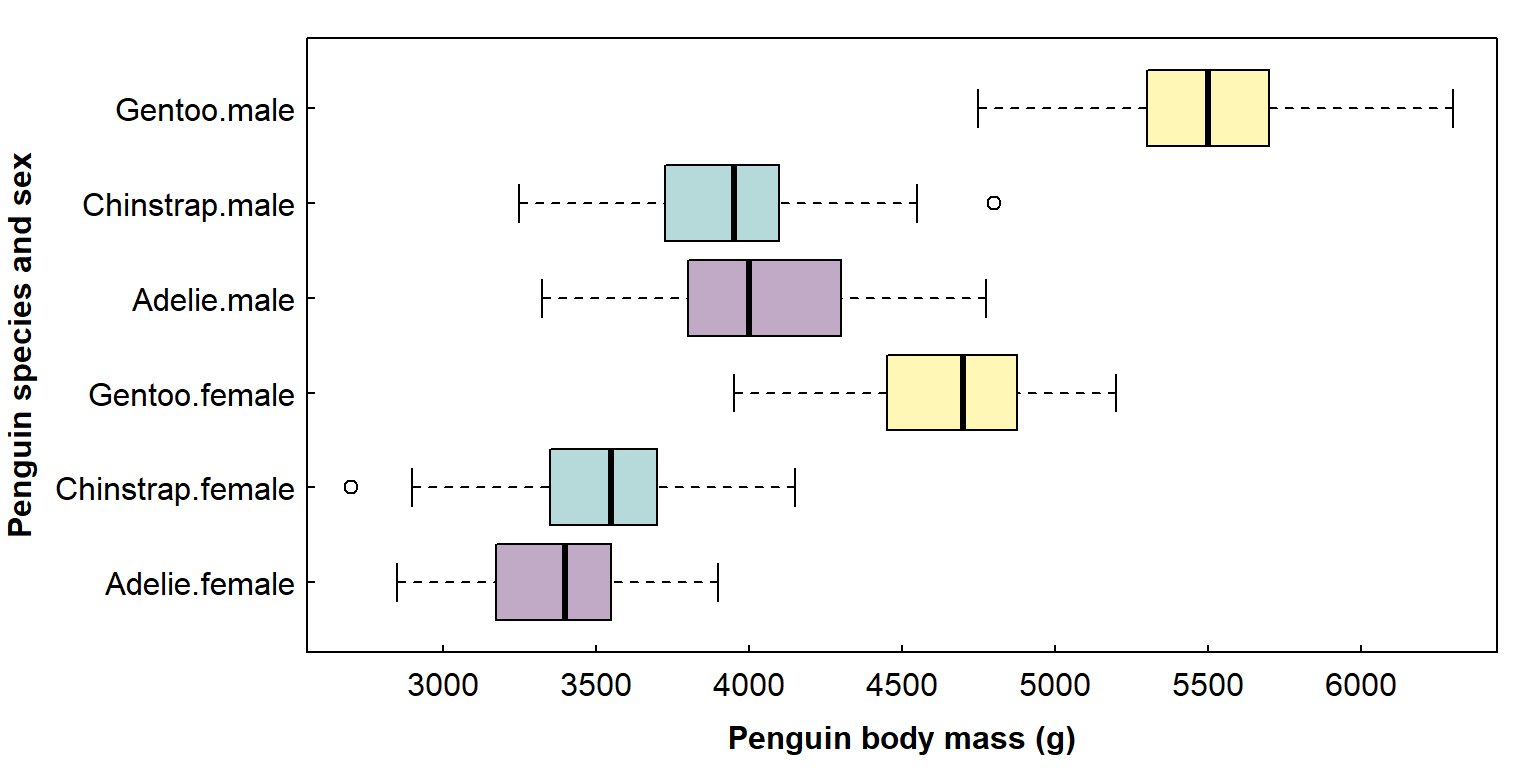
Hiding the code
To hide just the code, but display the output (text-based output,
plots, etc.), we include the option echo=FALSE. In
reports, we normally don't want to display the code or any warnings or
messages, so we could include all these options in each chunk:
par(mar=c(3,3,1,1), mgp=c(1.7,0.3,0), tcl=0.2)
# penguins is a built-in R dataset
with(penguins, boxplot(body_mass ~ species*sex, col=rep(2:4, 2), horizontal = TRUE,
las = 1, xlab="Penguin body mass (g)", ylab=""))
mtext("Penguin species and sex", side=2, line=7, font=2)
```
☝ this code would not appear in the knitted document since
echo=FALSE ☝
A more efficient way to do this, however, would be to modify the chunk at the beginning of our markdown when we create a new R markdown file in R:
knitr::opts_chunk$set(echo=FALSE, warning=FALSE, message=FALSE)
```
If we set these chunk options at the beginning, we can omit the
options echo=FALSE, warning=FALSE, message=FALSE in our
individual code chunks. We can override them if we want, e.g.
by including echo=TRUE.
Hiding the output
In assignments, we may want to display the code so that our Professor
or other person assessing our work can see that we know what to do,
without cluttering the assignment with lots of similar-looking output.
To hide just the output, but display the code (text-based output, plots,
etc.), we include the option results='hide'.
# penguins is a built-in R dataset (really!)
# check the contents of penguins dataset
print(penguins)
```
Re-sizing plots
One of the most useful sets of chunk options allows to change how
plots appear, such as fig.width, fig.height,
fig.align, and so on. For example, we could use
fig.width and fig.height make the previous
plot taller:
⋮
```
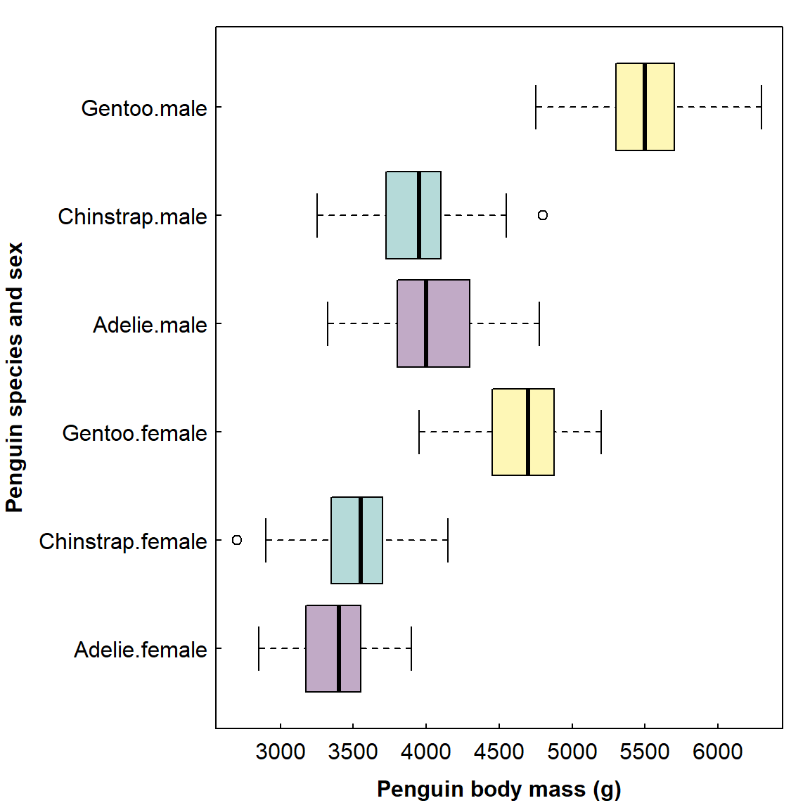
Setting fig.width and fig.height is for the
whole plot area so, if we have a multiple-frame plot (i.e.
using mfrow= or mfcol= in the
par() function), we would need to adjust the dimensions to
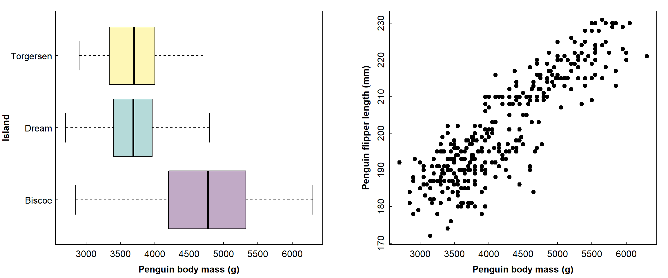
match. For example, the plots below show penguin body mass on three
islands (left), and penguin flipper length as a function of body mass
(right):
par(mfrow=c(1,2), mar=c(3,5,1,1), mgp=c(1.7,0.3,0), tcl=0.2, font.lab=2)
# penguins is a built-in R dataset
with(penguins, boxplot(body_mass ~ species*sex, col=rep(2:4, 2), horizontal = TRUE,
las = 1, xlab="Penguin body mass (g)", ylab=""))
mtext("Penguin species and sex", side=2, line=7, font=2)
with(penguins, plot(flipper_len ~ body_mass, pch = 19,
las = 0, xlab = "Penguin body mass (g)", ylab="Penguin flipper length (mm)"))
```
☝ this code would not appear in the knitted document since
echo=FALSE ☝
Adding figure captions to plots
We add captions using
fig.caption="<figure caption text>". This is a better
option for reporting than including a title above plots using the
main= option
ggplot(penguins[-which(is.na(penguins$sex)),]) +
geom_boxplot(aes(x=sex,y=bill_len, fill=sex)) +
scale_fill_manual(values=c("coral", "skyblue")) +
labs(x="Penguin sex", y="Bill length (mm)") +
facet_wrap(vars(species)) +
theme_bw()
```
☝ this code would not appear in the knitted document since
echo=FALSE ☝
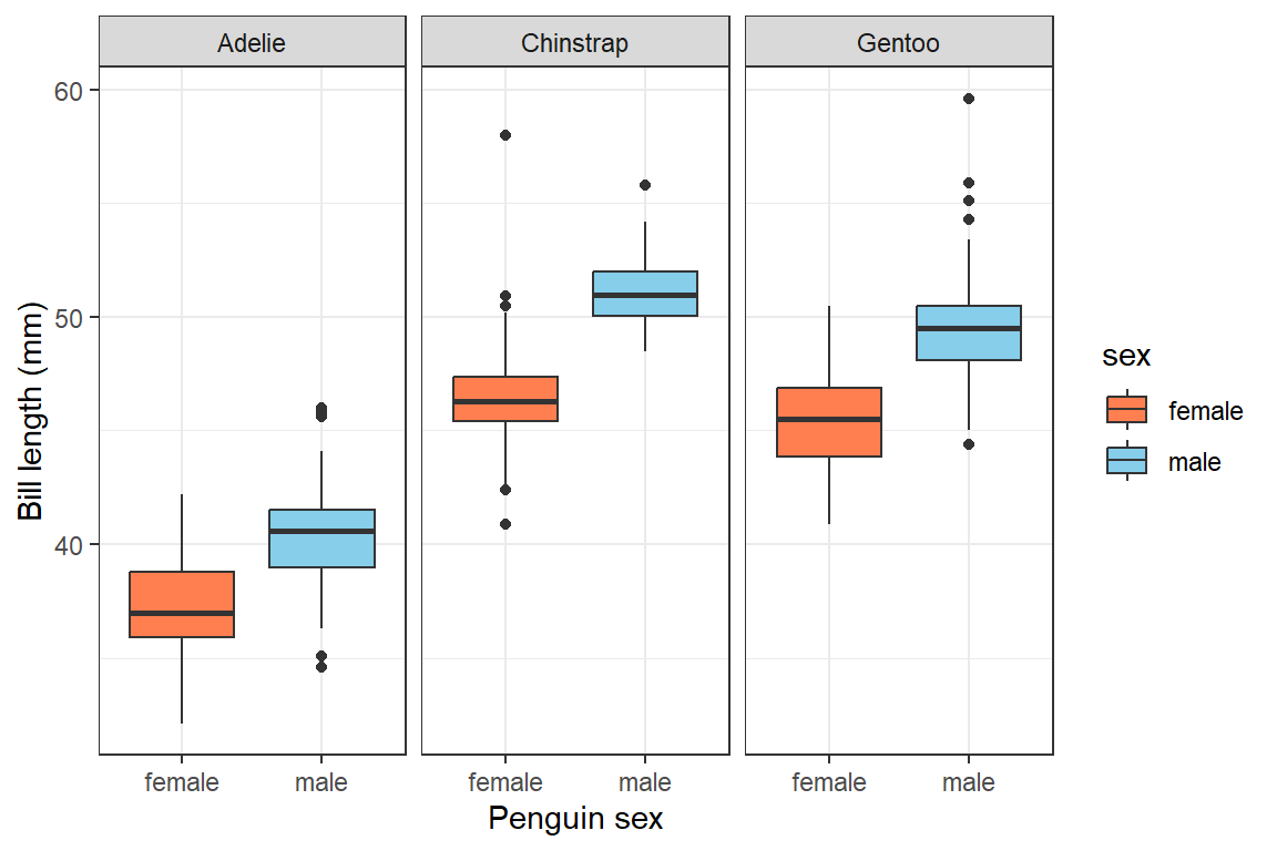
Figure 1: Penguin bill length by sex for three different penguin species.
We could just use normal markdown text to insert a caption, but using
fig.caption can allow automatic cross-referencing of
figures and tables to their captions using the bookdown R
package. 
At this stage it's useful to note that with a long chunk header
(within {}), such as that shown above, we should not insert
any line breaks. The chunk will return an error and not work unless
there are no line breaks in the chunk header.
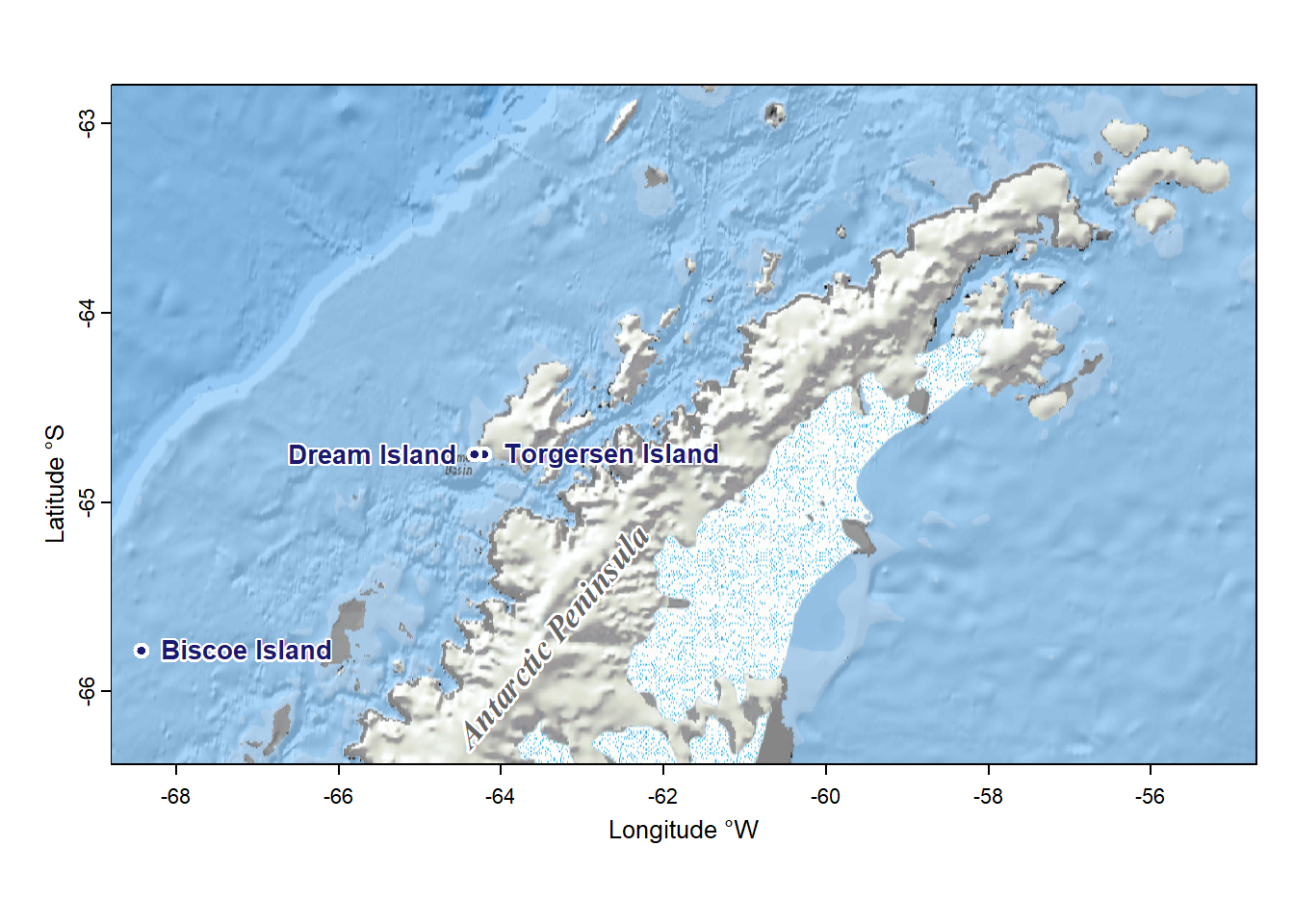
Figure 2: Locations of tiny Antarctic Islands where penguin data were collected.
Using the litedown package
I use the litedown package (Xie, 2025) as it's faster to
knit documents than rmarkdown with knitr, the
knitted files work well with my University's online Learning Management
System, and cross-referencing is simpler than when using the
bookdown package (see below).
litedown is designed to knit just to html, but this need
not be a limitation since apps like Microsoft Word can read html files
and (if desired) covert to pdf.
Setting up R markdown to knit with litedown
To make litedown the default knitting package, we need
to insert a line of yaml code into the R markdown file
yaml header:
⁝
knit: litedown:::knit
⁝
Cross-referencing with litedown
If we include a caption in the chunk options using
fig.cap =, this will automatically produce a numbered
caption if we knit our R markdown file with litedown. We
can then cross-reference using the chunk name prefixed with
@fig: for figures, @tab: for tables,
etc.
For this chunk:
⁝
```
...we would cross-reference the figure something like this:
Variations in penguin bill length are presented in @fig:penguins-plot-caption....to give the following text:
Variations in penguin bill length are presented in Figure 1.
For the best detail see https://yihui.org/litedown/#sec:cross-references
Automatic date when knitting with litedown
It could be just me, but I couldn't get an automatic date to work
using litedown if I included
date: "՝r Sys.Date()՝" in the yaml header. As
a workaround, I included an R code chunk like this:
cat("Andrew Rate, School of Agriculture and Environment, ", as.character(Sys.Date()))
```
Andrew Rate, School of Agriculture and Environment, 2025-12-04
Including the chunk option results='asis' means the
output will be treated as html when knitting, and the leading
# characters which usually precede text output are removed
with the comment="" option.
Using the bookdown package
The R package bookdown is very powerful, but so far I
only use it for its ability to provide automatic Figure and Table
numbering, and cross-referencing.
You would need to run the following R code if you don't have
bookdown installed:
You would also need to include the following in the yaml
header at the top of your R markdown document:
---
⋮
output:
  bookdown::html_document2:
⋮
---
This should give a menu option to
Knit to html_document2, which is what we should use later
to prepare our formatted document.
We can then use chunk names to cross reference figures and tables. For example, for the chunk above plotting two figures...
⁝
```
...we would cross-reference this by including
Figure \@ref(fig:penguins-two-plots) at the appropriate
place in our text.
Notes
- chunk names can not contain spaces, periods, underscores, or
slashes; words should just be separated by hyphens (
-), and all chunk names must be unique - we don't need to include the word
Figureor a figure number at the start of thefig.cap=text string in the chunk header ({r . . . })
Similarly, table captions can be cross-referenced using
Table \@ref(tab:table-chunk-name) in the text outside of
any code chunks. We would need to set a table caption in the chunk
header using tab.cap=, or use a package like
flextable or knitr::kable() and include table
caption options from those packages.
Other chunk options
Option | Purpose |
|---|---|
out.width= | Sets the width of a figure as a proportion of the output page width, |
fig.align= | Aligns the figure on the output page |
results='hold' | Waits until all the code in a chunk has run before printing any text output |
paged.print= | If TRUE (the default) adds html format to printed data frames; |
You can see a more complete table in the R Markdown Cheatsheet.
Other R Markdown Resources
R Markdown Cheat Sheet (Posit Software, 2024)
Getting used to R, RStudio, and R Markdown – Chapter 4 in the excellent (and free) eBook by Chester Ismay
Chunk Options – Chapter 11 in R markdown cookbook by Xie et al. (2025)
The
litedownpackage by Yihui Xie – “...an attempt to reimagine R Markdown with one primary goal — do HTML, and do it well, with the minimalism principle.”
References
Ismay, Chester (2016) Getting used to R, RStudio, and R Markdown. https://bookdown.org/chesterismay/rbasics/ (accessed 2025-06-17)
Posit Software (2024) rmarkdown:: CHEATSHEET.
https://rstudio.github.io/cheatsheets/rmarkdown.pdf
(accessed 2025-06-17)
Xie, Yihui (2020) Chunk Options and Package Options. https://yihui.org/knitr/options/ (accessed 2025-06-17)
Xie Y (2025). knitr: A General-Purpose Package for
Dynamic Report Generation in R. R package version 1.50, https://yihui.org/knitr/.
Xie Y (2025). litedown: A Lightweight Version of R
Markdown. doi:10.32614/CRAN.package.litedown, R package
version 0.7, https://CRAN.R-project.org/package=litedown.
Xie Y, Dervieux C, Riederer E (2025) R Markdown Cookbook. https://bookdown.org/yihui/rmarkdown-cookbook/ (accessed 2025-06-17)
CC-BY-SA • All content by Ratey-AtUWA. My employer does not necessarily know about or endorse the content of this website.
Created with rmarkdown in RStudio. Currently using the free yeti theme from Bootswatch.