 Material to support teaching in Environmental Science at The University of Western Australia
Units ENVT3361, ENVT4461, and ENVT5503
Statistical Relationships
Grouped linear regression
Andrew Rate
2025-12-05
Relationships pages: Correlations | Simple linear regression | Grouped linear regression | Multiple linear regression
Suggested activities
Using the R code file provided and the afs1923
dataset:
- Run a grouped regression model,
- Assess whether or not the grouped regression model meets the statistical assumptions,
- Evaluate whether a grouped regression model is a statistically significant improvement on the comparable ungrouped model, and
- Make sure you understand the concepts for all the statistical methods you use, and can interpret all the output!
Introduction
In a previous session on simple regression, we finished by suggesting that one way we could make regression prediction more accurate was by
allowing regression relationships to differ for different groups in our data (defined by a factor variable) – regression by groups
This session will continue or efforts to predict Cr from Al, but we know the data were derived from analysis of samples from diverse types of environment. For that reason, it seems reasonable to evaluate a regression model which allows the regression coefficients (intercept and slope) to differ for different sample types.
As previously, our first step is to read the data, and change anything we need to:
git <- "https://github.com/Ratey-AtUWA/Learn-R-web/raw/main/"
afs1923 <- read.csv(paste0(git,"afs1923.csv"), stringsAsFactors = TRUE)
# re-order the factor levels
afs1923$Type <- factor(afs1923$Type, levels=c("Drain_Sed","Lake_Sed","Saltmarsh","Other"))
afs1923$Type2 <-
  factor(afs1923$Type2,
         levels=c("Drain_Sed","Lake_Sed","Saltmarsh W","Saltmarsh E","Other"))
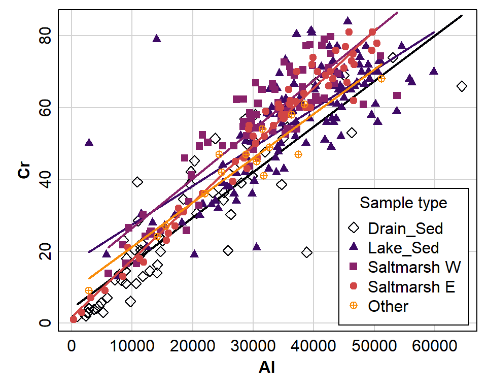
Next, we inspect a scatterplot of the variables which matches the kind of regression model we intend to apply (Figure 1):
library(car)
par(mar=c(3,3,0.5,0.5), mgp=c(1.3,0.2,0), tcl=0.2, font.lab=2)
scatterplot(Cr ~ Al | Type2, data=afs1923, smooth=FALSE,
            col=inferno(nlevels(afs1923$Type2), end=0.75), pch=c(5,17,15,19,10),
            legend=list(coords="bottomright", title="Sample type"))
Figure 1: Different relationships predicting Cr from Al depending on the sample type (data from analysis of sediments from Ashfield Flats, 2019-2023.
Predicting chromium from aluminium using a regression model which varies by groups
Note the syntax used to separate by factor categories:
##
## Call:
## lm(formula = Cr ~ Al * Type2, data = afs1923)
##
## Residuals:
##     Min      1Q  Median      3Q     Max
## -33.644  -5.039  -0.195   4.637  47.183
##
## Coefficients:
##                       Estimate Std. Error t value Pr(>|t|)
## (Intercept)          4.069e+00  1.845e+00   2.205  0.02813 *
## Al                   1.268e-03  7.872e-05  16.114  < 2e-16 ***
## Type2Lake_Sed        1.264e+01  3.166e+00   3.994 8.04e-05 ***
## Type2Saltmarsh W     8.628e+00  3.507e+00   2.460  0.01440 *
## Type2Saltmarsh E    -2.367e+00  3.366e+00  -0.703  0.48231
## Type2Other           4.806e+00  6.162e+00   0.780  0.43600
## Al:Type2Lake_Sed    -1.928e-04  1.036e-04  -1.861  0.06362 .
## Al:Type2Saltmarsh W  1.056e-04  1.209e-04   0.873  0.38318
## Al:Type2Saltmarsh E  3.282e-04  1.140e-04   2.880  0.00424 **
## Al:Type2Other       -3.437e-05  2.091e-04  -0.164  0.86954
## ---
## Signif. codes:  0 '***' 0.001 '**' 0.01 '*' 0.05 '.' 0.1 ' ' 1
##
## Residual standard error: 8.444 on 325 degrees of freedom
## Multiple R-squared:  0.8362, Adjusted R-squared:  0.8317
## F-statistic: 184.4 on 9 and 325 DF,  p-value: < 2.2e-16
This is similar output to simple linear regression in the previous
example, but the Coefficients: table is much more
complicated.
- The first two rows of the
Coefficients:table under the headings give the intercept and slope for the 'base case', which by default is the first group in the factor separating the groups. In this example the first level of the factorTypeisDrain_Sed(frustratingly, the output does not show this). - The next 4 rows, starting with the factor name (i.e.
Type2Lake_Sed, etc.), show the difference between the intercepts forLake_Sed,Saltmarsh W,Saltmarsh E, andOthergroups compared with the base case. - Similarly, the final rows, beginning with the predictor variable
name (
Al:Type2Lake_Sed,Al:Type2Saltmarsh W,Al:Type2Saltmarsh E, andAl:Type2Other), show the difference between the slopes forLake_Sed,Saltmarsh W,Saltmarsh E, andOthergroups compared with the base case (shown asAlbut actually the slope for theDrain_Sedgroup).
Compare the two models
Sometimes models can have greater R2 but only because
we've made them more complex by grouping our observations or by adding
more predictors. We want the simplest model possible.
We compare the models using an analysis of variance with the
anova() function (where the null hypothesis is equal
predictive ability). The models compared need to be
nested, that is, one is a subset of the other.
Before we do this, we need to re-create the simple model from a previous session:
##
## Call:
## lm(formula = Cr ~ Al, data = afs1923)
##
## Residuals:
##     Min      1Q  Median      3Q     Max
## -40.751  -5.349  -0.251   5.774  52.250
##
## Coefficients:
##              Estimate Std. Error t value Pr(>|t|)
## (Intercept) 7.672e+00  1.284e+00   5.976 5.89e-09 ***
## Al          1.359e-03  3.829e-05  35.480  < 2e-16 ***
## ---
## Signif. codes:  0 '***' 0.001 '**' 0.01 '*' 0.05 '.' 0.1 ' ' 1
##
## Residual standard error: 9.428 on 333 degrees of freedom
## Multiple R-squared:  0.7908, Adjusted R-squared:  0.7902
## F-statistic:  1259 on 1 and 333 DF,  p-value: < 2.2e-16
So our more complex (grouped) linear model has greater R2
(0.836) than the simple linear model (R2 = 0.791). We now
perform the anova test to see whether this improvement is
significant:
## Analysis of Variance Table
##
## Model 1: Cr ~ Al
## Model 2: Cr ~ Al * Type2
##   Res.Df   RSS Df Sum of Sq      F    Pr(>F)
## 1    333 29599
## 2    325 23174  8    6424.7 11.263 4.366e-14 ***
## ---
## Signif. codes:  0 '***' 0.001 '**' 0.01 '*' 0.05 '.' 0.1 ' ' 1
The p-value (Pr(>F)) is ≃ 4.4×10⁻¹⁴,
i.e. below 0.05, so we reject H0 that the models
have equivalent predictive ability. In that case the model which
explains more variance in the dependent variable Cr is
best; that is, the grouped linear model with
R2 = 0.836 (i.e., explaining 83.6% of the variance
in Cr based on the variance in Al divided into
groups by the factor Type2).
The choice of models should be based on an interpretation of “Occam's Razor” a.k.a. the “Principle of Parsimony”:
“Plurality must never be posited without necessity.”
— William of Ockham (also spelled Occam) (1285 - 1348), English theologian, logician, and Franciscan friar
In practice this means that if more than one hypothesis or model explains our data equally well, we should always choose the simplest one.
Another way we can test for the most appropriate model is by using the AIC or Aikake Information Criterion, which ‘penalises’ a model having more parameters. A better model will have a lower value of AIC, and the built-in penalty means that for equivalent models (i.e. non-significant ANOVA) the model with more parameters will have greater AIC, and so we should select the simpler model with the least AIC value. For our two models, AIC should still be lower for the more complex model (otherwise we are in trouble, since the ANOVA and AIC would disagree, and then which one would we choose?). Anyway, let's find out:
##               df      AIC
## lmCrAlsimple   3 2457.942
## lmCrAl_byType 11 2391.968
The output from the AIC() function shows that even
though the degrees of freedom df for the grouped model (11)
is much greater than for the simple model (3), the grouped model still
has a lower AIC value (≃2392) than the simple model (≃2456). So, the
ANOVA and AIC do agree after all 😌.
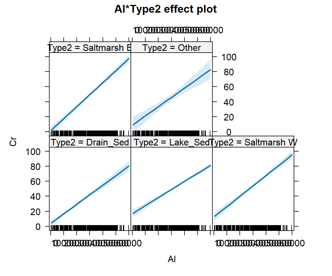
We can see a little more detail about the individual group-wise
relationships or ‘effects’ by plotting an effects plot using functions
from the effects package (Figure 2):

Figure 2: Effect plots showing the effects of interacting predictors
Al * Type2 on Cr, using data from sediments at Ashfield
Flats 2019-2023.
So even though the plots in Figure 1 and Figure 2 suggest that each
group has a similar Cr ~ Al relationship, the slopes and
intercepts differ enough between groups to give an improved prediction
over the simple model.
Regression assumptions
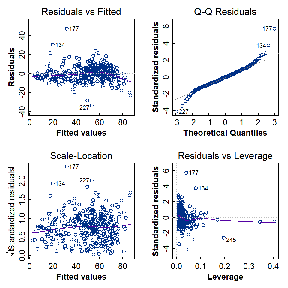
The assumptions implicit in linear regression were presented in the session on simple linear regression models. We run the same set of diagnostic tests on more complex regression models as well.
Formal statistical tests of regression assumptions
As with simple linear regression, we can test all of the assumptions with formal statistical tests (see the simple linear regression session for explanations and null hypotheses).
##
##  Shapiro-Wilk normality test
##
## data:  lmCrAl_byType$residuals
## W = 0.95798, p-value = 3.26e-08##
## Breusch-Godfrey test for serial correlation of order up to 1
##
## data: lmCrAl_byType
## LM test = 52.363, df = 1, p-value = 4.613e-13##
## studentized Breusch-Pagan test
##
## data: lmCrAl_byType
## BP = 36.366, df = 9, p-value = 3.413e-05##
## Rainbow test
##
## data: lmCrAl_byType
## Rain = 0.51147, df1 = 168, df2 = 157, p-value = 1## rstudent unadjusted p-value Bonferroni p
## 177 6.003042 5.1884e-09 1.7381e-06
## 227 -4.192086 3.5701e-05 1.1960e-02## Min. 1st Qu. Median Mean 3rd Qu. Max.
## 1.000e-09 1.556e-04 7.584e-04 3.602e-03 2.223e-03 1.663e-01infl.lmCrAl <- influence.measures(lmCrAl_byType)
ninf <- nrow(summary(infl.lmCrAl)) # number of possibly influential observations
modform <- deparse(lmCrAl_byType$call)
rninf <- row.names(summary(infl.lmCrAl)) # IDs of possibly influential observations
# if you run this code chunk yourself you will see the whole summary(infl.lmCrAl) outputcat(paste0("For the model '", modform, "' there are ", ninf,
" potentially influential observations.\n\n"))
cat("The", ninf, "rows containing potentially influential obervations are:\n"); as.integer(rninf)## For the model 'lm(formula = Cr ~ Al * Type2, data = afs1923)' there are 36 potentially influential observations.
##
## The 36 rows containing potentially influential obervations are:
## [1] 2 56 92 134 137 138 139 168 177 190 196 218 219 220 227 236 245 250 251 252 273 290 291 296 297 298 316 317 318
## [30] 319 320 321 322 323 324 325To summarise:
Test | Assessing | Results |
|---|---|---|
Shapiro-Wilk | Are residuals normally distributed? | No (qq-plot suggests long tails) |
Breusch-Godfrey | Are residuals independent? | No, there is autocorrelation |
Breusch-Pagan | Are residuals homoscedastic? | No (p<0.05) |
Rainbow | Is the relationship linear? | Yes (p>0.05) |
Outlier | Are there significant outliers (Bonferroni)? | 2 points are possible outliers |
Cook's Distance | Are there any potentially influential observations? | No (no values > 0.5) |
Infuence Measures | Are there any potentially influential observations? | Yes (36 out of 335 observations) |
The summary of the diagnostic tests in Table 1 shows that not all the formal assumptions of regression are fulfilled by our model. Even though the model may not be strictly statistically valid, the regression output showed that ≃ 84% of the variance in Cr could be explained by Al when observations were grouped by sample type. So, from a practical perspective, this grouped regression model could also be used for prediction, and the greater R2 makes it a better prediction option than the simple model discussed in another session.
The next option would be a model which has more than one predictor variable for our dependent variable – multiple regression.
