 Material to support teaching in Environmental Science at The University of Western Australia
Units ENVT3361, ENVT4461, and ENVT5503
Utilities = useful stuff
Making use of unusual regression residuals
Andrew Rate
2025-12-05
Do large positive regression residuals indicate contamination?
Background concentrations of contaminants are usually defined as being concentrations which occur naturally, in the absence of additions derived from human activity. It is generally recognised that:
- background concentrations in water, sediments, and soils vary spatially, depending on the local geology, the age of the landscape in which a site under investigation is situated, etc. (Reimann and Garrett, 2005)
- background concentrations of contaminants in soils and sediments are not a single constant value, but are instead a function of sediment properties such as pH, cation exchange capacity, or the concentrations of major elements such as Al, Fe, or Mn (Hamon et al., 2004)
library(car)           # Companion to Applied Regression
library(sf)            # Simple Features spatial data in R
library(maptiles)      # get open-source map tiles for background maps
library(prettymapr)    # add scale bar and north arrows to maps
For this session we're going to use the Ashfield Flats compiled data from 2019-2023.
git <- "https://github.com/Ratey-AtUWA/Learn-R-web/raw/main/"
afs1923 <- read.csv(paste0(git,"afs1923.csv"), stringsAsFactors = TRUE)
# re-order the factor levels
afs1923$Type <- factor(afs1923$Type, levels=c("Drain_Sed","Lake_Sed","Saltmarsh","Other"))
afs1923$Type2 <-
  factor(afs1923$Type2,
         levels=c("Drain_Sed","Lake_Sed","Saltmarsh W","Saltmarsh E","Other"))
afr_map <-
  read.csv("https://raw.githubusercontent.com/Ratey-AtUWA/spatial/main/afr_map_v2.csv",
           stringsAsFactors = TRUE)
extent <- st_as_sf(data.frame(x=c(399900,400600),y=c(6467900,6468400)),
                   coords = c("x","y"), crs = UTM50S)
aftiles <- get_tiles(extent, provider = "CartoDB.Voyager", crop = TRUE)
It's good practice to remove missing observations from the data we
use to generate our multiple regression model. This is usually
essential practice when conducting multiple regression,
since if the stepwise procedure removes or adds predictors, successive
iterations of the stepwise refinement procedure may need to use a
different number of observations, which will cause an error. See the
Warning and other information at help(step) for more
detail. We're also log10-transforming positively skewed
variables, in an effort to address later issues with the distribution
and variance of linear model residuals.
regdata <- na.omit(afs1923[,c("Pb","pH","Al","Ca","Fe","S","P","Na","K","Mg")])
regdata$Pb.log <- log10(regdata$Pb)
regdata$Ca.log <- log10(regdata$Ca)
regdata$S.log <- log10(regdata$S)
regdata$P.log <- log10(regdata$P)
regdata$Na.log <- log10(regdata$Na)
regdata$Mg.log <- log10(regdata$Mg)
row.names(regdata) <- NULL
cat("original data has",nrow(afs1923),"rows, subset has",nrow(regdata),"rows\n\n")
## original data has 335 rows, subset has 298 rowscors <- cor(regdata[,c("Pb.log","pH","Al","Ca.log","Fe","S.log","P.log",
"Na.log","K","Mg.log")])
cors[which(cors==1)] <- NA
print(cors, digits=2, na.print = "")## Pb.log pH Al Ca.log Fe S.log P.log Na.log K Mg.log
## Pb.log 0.102 0.381 0.239 0.418 0.216 0.726 0.33 0.34 0.437
## pH 0.10 -0.121 0.322 0.068 0.068 0.035 -0.11 -0.12 0.031
## Al 0.38 -0.121 0.096 0.244 0.017 0.246 0.51 0.76 0.645
## Ca.log 0.24 0.322 0.096 0.210 0.350 0.452 0.24 0.17 0.380
## Fe 0.42 0.068 0.244 0.210 0.354 0.615 0.44 0.33 0.497
## S.log 0.22 0.068 0.017 0.350 0.354 0.423 0.45 0.27 0.426
## P.log 0.73 0.035 0.246 0.452 0.615 0.423 0.49 0.36 0.546
## Na.log 0.33 -0.106 0.512 0.238 0.440 0.454 0.491 0.76 0.933
## K 0.34 -0.118 0.759 0.174 0.329 0.268 0.361 0.76 0.795
## Mg.log 0.44 0.031 0.645 0.380 0.497 0.426 0.546 0.93 0.79
From the correlation matrix above, we notice that Na, Mg are
correlated with r = 0.933 (definitely r>0.8), so Na and Mg are too
collinear. We therefore omit one of this collinear pair from our initial
model. We add spatial coordinates (Easting,
Northing) to the data subset, not to include them in models
but because we'll use them later.
regdata <- na.omit(afs1923[,c("Pb","pH","Al","Ca","Fe","S","P","Na","K","Easting","Northing")])
row.names(regdata) <- NULL
regdata$Pb.log <- log10(regdata$Pb)
regdata$Ca.log <- log10(regdata$Ca)
regdata$S.log <- log10(regdata$S)
regdata$P.log <- log10(regdata$P)
regdata$Na.log <- log10(regdata$Na)
cat("original data has",nrow(afs1923),"rows, subset has",nrow(regdata),"rows")
## original data has 335 rows, subset has 298 rowsIt's always good practice to check scatterplots of the potential relationships too, to make sure there are no odd apparent relationships caused by outliers or clustering of points (this is more of an issue when we have fewer observations).
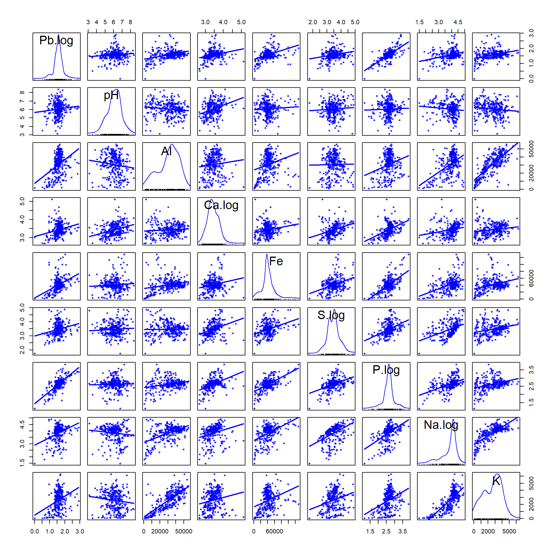
Figure 1: Scatter plot matrix for Pb and potenial multiple regression predictors. Positively skewed variables are log10-transformed.
The scatter plot matrix (Figure 1) is useful for showing whether the
relationships between the dependent variable (Pb) and
individual predictors has (i) any outliers that might influence
regression parameters, or; (ii) if there is any clustering apparent. The
first row (horizontal) of the scatter plot matrix is particularly useful
because it shows the relationship of our dependent variable
(Pb) vs. each of the individual predictors.
We should also run the correlation matrix again:
cors <- cor(regdata[,c("Pb.log","pH","Al","Ca.log","Fe","S.log","P.log","Na.log","K")])
cors[which(cors==1)] <- NA
print(signif(cors,2), na.print = "")
## Pb.log pH Al Ca.log Fe S.log P.log Na.log K
## Pb.log 0.100 0.380 0.240 0.420 0.220 0.730 0.33 0.34
## pH 0.10 -0.120 0.320 0.068 0.068 0.035 -0.11 -0.12
## Al 0.38 -0.120 0.096 0.240 0.017 0.250 0.51 0.76
## Ca.log 0.24 0.320 0.096 0.210 0.350 0.450 0.24 0.17
## Fe 0.42 0.068 0.240 0.210 0.350 0.620 0.44 0.33
## S.log 0.22 0.068 0.017 0.350 0.350 0.420 0.45 0.27
## P.log 0.73 0.035 0.250 0.450 0.620 0.420 0.49 0.36
## Na.log 0.33 -0.110 0.510 0.240 0.440 0.450 0.490 0.76
## K 0.34 -0.120 0.760 0.170 0.330 0.270 0.360 0.76The revised correlation matrix above shows no r values above 0.8, but some close to the r=0.8 threshold (e.g. Al-K r=0.76; Na-K r=0.76). We will need to check the variance inflation factors one we have run the initial model.
##
## Call:
## lm(formula = Pb.log ~ pH + Al + Ca.log + Fe + S.log + P.log +
##     Na.log + K, data = regdata)
##
## Residuals:
##      Min       1Q   Median       3Q      Max
## -0.57663 -0.11881 -0.01945  0.09097  0.96958
##
## Coefficients:
##               Estimate Std. Error t value Pr(>|t|)
## (Intercept) -2.516e-01  1.723e-01  -1.460 0.145405
## pH           6.127e-02  1.561e-02   3.925 0.000108 ***
## Al           8.283e-06  1.505e-06   5.505 8.15e-08 ***
## Ca.log      -1.696e-01  4.430e-02  -3.828 0.000159 ***
## Fe          -1.571e-06  8.327e-07  -1.886 0.060269 .
## S.log        1.730e-04  3.314e-02   0.005 0.995838
## P.log        8.192e-01  5.102e-02  16.055  < 2e-16 ***
## Na.log      -7.348e-02  3.556e-02  -2.066 0.039687 *
## K           -8.771e-06  1.875e-05  -0.468 0.640334
## ---
## Signif. codes:  0 '***' 0.001 '**' 0.01 '*' 0.05 '.' 0.1 ' ' 1
##
## Residual standard error: 0.2118 on 289 degrees of freedom
## Multiple R-squared:  0.6232, Adjusted R-squared:  0.6128
## F-statistic: 59.74 on 8 and 289 DF,  p-value: < 2.2e-16
The regression output shows that we can't reject the null hypothesis of no effect for several variables. This may be due to our model being over-parameterised, and we hope that we can rely on the stepwise selection procedure to eliminate unnecessary predictors. Let look at the VIF values:
##       pH       Al   Ca.log       Fe    S.log    P.log   Na.log        K
## 1.193383 2.628976 1.520550 1.751400 1.563434 2.154061 3.079927 4.257511
None of the VIF values indicate that predictors should be removed, but the value > 4 (4.26 for K) is worth remembering when we generate the final model by stepwise parameter selection.
That's what we do next, using the step() function. If
we're being really careful, we can compare different options for
generating a multiple regression model, e.g.:
direction = "forward"– starting from a minimal model and successively adding predictors;direction = "backward"– starting from a maximal model and successively removing predictors;direction = "both"(the default is"both", which we have used) – specifying a maximal model and allowing and testing addition and removal of predictors.
If we're interested in seeing some of the progress of the stepwise
algorithm, we can specify trace=1. See
help(step) for more detail.
##
## Call:
## lm(formula = Pb.log ~ pH + Al + Ca.log + Fe + P.log + Na.log,
##     data = regdata)
##
## Residuals:
##      Min       1Q   Median       3Q      Max
## -0.57968 -0.11802 -0.01794  0.09023  0.96002
##
## Coefficients:
##               Estimate Std. Error t value Pr(>|t|)
## (Intercept) -2.222e-01  1.553e-01  -1.431 0.153501
## pH           6.135e-02  1.556e-02   3.943 0.000101 ***
## Al           7.831e-06  1.081e-06   7.245 3.88e-12 ***
## Ca.log      -1.700e-01  4.333e-02  -3.922 0.000109 ***
## Fe          -1.561e-06  8.249e-07  -1.893 0.059359 .
## P.log        8.195e-01  5.060e-02  16.195  < 2e-16 ***
## Na.log      -8.339e-02  2.678e-02  -3.114 0.002030 **
## ---
## Signif. codes:  0 '***' 0.001 '**' 0.01 '*' 0.05 '.' 0.1 ' ' 1
##
## Residual standard error: 0.2111 on 291 degrees of freedom
## Multiple R-squared:  0.6229, Adjusted R-squared:  0.6151
## F-statistic: 80.11 on 6 and 291 DF,  p-value: < 2.2e-16
Check the AIC for the maximal and stepwise models...
##     df       AIC
## lm0 10 -68.60634
## lm1  8 -72.37964
...and check the VIF for the predictors:
##       pH       Al   Ca.log       Fe    P.log   Na.log
## 1.193117 1.365100 1.464100 1.729388 2.131921 1.757584
Our final model has six predictors, reduced from eight in the maximal model. [We could even try a model without Fe as a predictor, since we can't reject H0 for Fe based on its p-value ≃0.06. Since it's marginal we'll leave it in for now...]. Based on its lower AIC value, the stepwise model provides a better combination of predictive ability and parsimony than the maximal model. The stepwise refinement has removed K and S as predictors, so we no longer have any issue with collinearity. It's interesting to compare the regression coefficients with the individual correlation coefficients:
(r_vs_coefs <- data.frame(Pearson_r=cors[names(lm1$coefficients[-1]),1],
                         lm_coefs=lm1$coefficients[-1]))
## Pearson_r lm_coefs
## pH 0.1023659 6.134560e-02
## Al 0.3807144 7.831464e-06
## Ca.log 0.2391211 -1.699679e-01
## Fe 0.4176609 -1.561546e-06
## P.log 0.7260967 8.195048e-01
## Na.log 0.3282740 -8.338841e-02We can see that all the correlation coefficients are
positive, but that the regression coefficients for Ca, Fe, and
Na are negative.
In a multiple linear regression model, the effects of the predictors
interact, so we don't always see the effects we might expect based on
simple correlation.
par(mfrow=c(1,1), mgp=c(1.5,0.2,0), tcl=0.25, mar=c(3,3,0.5,0.5), las=1, lend="square", xpd=F)
plot(lm1$model$Pb.log ~ lm1$fitted.values,
     xlab=expression(bold(paste(log[10],"Pb predicted by model"))),
     ylab=expression(bold(paste("Observed ",log[10],"Pb"))),
     pch=19, cex=1.2, col="#0000ff40"); abline(0,1,col="sienna")
newdata <- data.frame(pH=seq(min(regdata$pH),max(regdata$pH),l=50),
                      Al=seq(min(regdata$Al),max(regdata$Al),l=50),
                      Ca.log=seq(min(regdata$Ca.log),max(regdata$Ca.log),l=50),
                      Fe=seq(min(regdata$Fe),max(regdata$Fe),l=50),
                      P.log=seq(min(regdata$P.log),max(regdata$P.log),l=50),
                      Na.log=seq(min(regdata$Na.log),max(regdata$Na.log),l=50))
conf0 <- predict(lm1, newdata, interval = "prediction", level=0.95)
lines(conf0[,1], conf0[,2], col="grey", lty=3, lwd=2)
lines(conf0[,1], conf0[,3], col="grey", lty=3, lwd=2)
legend("topleft", bty="n", inset=0.01, pt.cex=1.2, pch=c(19,NA,NA),
       legend=c("Observations","1:1 line","±95% prediction"),
       col=c("#0000ff40","sienna","grey"), lty=c(NA,1,3),lwd=c(NA,1,2))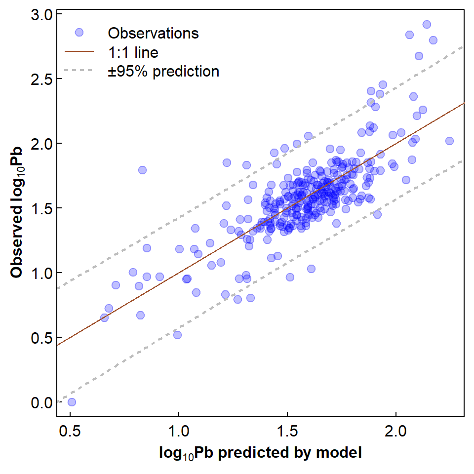
Figure 2: Relationship of observed to predicted log10-Pb showing 1:1 line and 95% prediction interval.
The observed vs. predicted log10Pb in Figure 2
shows the expected scatter about a 1:1 line, with some positive
residuals that may be unusually large. If we convert the residuals to
standard normal distribution scores (the R tool for this is the
scale() function) then we may be able to identify which
observations are unusually high, e.g. ≥ 2 standard deviations
above the mean.
par(mfrow=c(1,1), mgp=c(1.5,0.2,0), tcl=0.25, mar=c(3,3,0.5,0.5), las=1, lend="square", xpd=F)
boxplot(scale(lm1$residuals), col="lemonchiffon", xlab=expression(bold(paste(log[10],"Pb"))),
        ylab="Standardised residual from multiple regression model ")
#abline(h=2, col=4, lty=2)
rect(par("usr")[1],2,par("usr")[2],par("usr")[4],border="transparent", col="#00308720")
arrows(0.65,3.8,y1=par("usr")[4],angle = 20,length = 0.1, col="#003087")
arrows(0.65,2.8,y1=2,angle = 20,length = 0.1, col="#003087")
text(0.5, 3.2, pos=4, offset=0.2, col="#003087", cex=0.8,
     labels="Standardised\nresidual > 2\n(p \u2248 0.025)")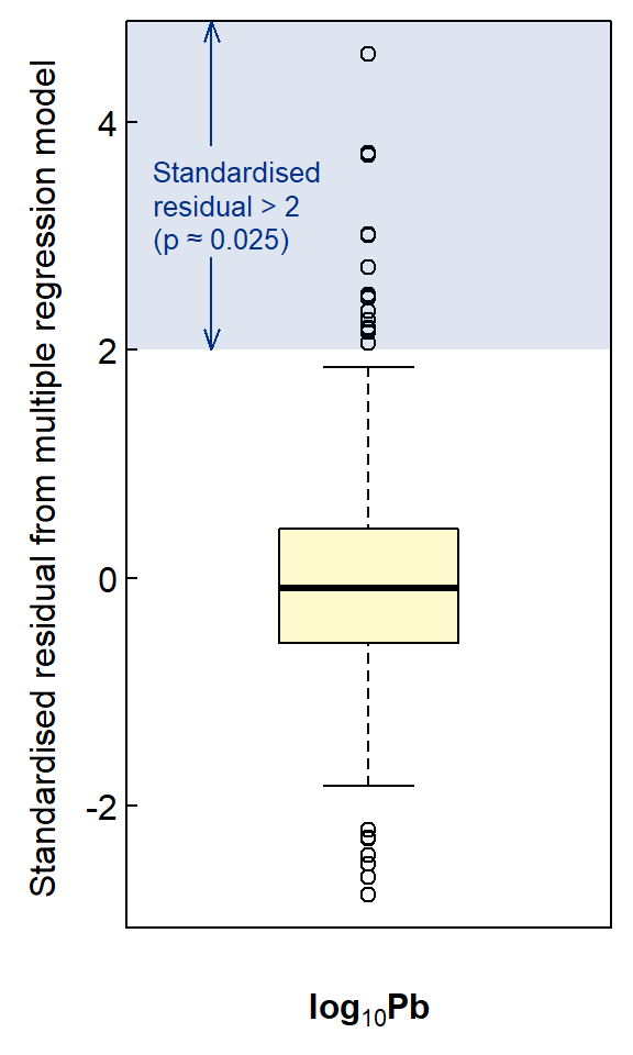
Figure 3: Box plot of model residuals scaled to standard normal distribution scores (mean=0, sd=1).
cat("---- Large log10(Pb) ----\n");lm1$model$Pb.log[which(scale(lm1$residuals)>=2)]
cat("\n---- Back-transformed ----\n");10^(lm1$model$Pb.log[which(scale(lm1$residuals)>=2)])
## ---- Large log10(Pb) ----
## [1] 1.850646 1.831870 2.316809 2.674677 2.919653 2.382737 1.929419 1.995635 1.961421 2.799134 2.838912 2.453318
## [13] 2.403635 1.792392 2.056905
##
## ---- Back-transformed ----
## [1] 70.9 67.9 207.4 472.8 831.1 241.4 85.0 99.0 91.5 629.7 690.1 284.0 253.3 62.0 114.0par(mfrow=c(1,1), oma=c(0,0,0,0), lend="square", xpd=TRUE)
plot_tiles(aftiles, adjust=F, axes=TRUE, mar=c(3,3,0.5,0.5)) # use axes = TRUE
mtext("Easting (UTM Zone 50, m)", side = 1, line = 3, font=2)
mtext("Northing (UTM Zone 50, m)", side = 2, line = 2.5, font=2)
addnortharrow(text.col=1, border=1, pos="topleft")
addscalebar(plotepsg = 32750, label.col = 1, linecol = 1,
label.cex = 1.2, htin=0.15, widthhint = 0.3)
with(afr_map, lines(drain_E, drain_N, col = "cadetblue", lwd = 2))
with(afr_map, polygon(wetland_E, wetland_N, col = "#5F9EA080",
border="cadetblue", lwd = 1, lty = 1))
text(c(400250, 399962, 400047), c(6468165, 6468075, 6468237),
labels = c("Chapman\nDrain","Kitchener\nDrain", "Woolcock\nDrain"),
pos = c(2,2,4), cex = 0.8, font = 3, col = "cadetblue")
with(regdata[which(scale(lm1$residuals)>=2),],
points(Easting, Northing, pch=21, col="#000000b0", bg="#ffe000b0", cex=1.4, lwd=2))
with(regdata[which(scale(lm1$residuals)>=2),],
text(Easting, Northing, labels=round(Pb,0), cex=0.8,
pos=c(2,4,2,1,4,2,4,4,4,3,4,4,4,2), offset=0.3))
legend("bottomright", box.col="#ffffff40", bg="#ffffff40", y.intersp=1.75,
legend=c("Sediment samples with \nPb standardised residuals ≥ 2",
"Numbers next to points are\nPb concentrations (mg/kg)"),
pch = c(21,NA), col = c("#000000b0","black"), pt.bg = "#ffe000b0",
inset = c(0.02,0.04), pt.cex=c(1.4,0.8), pt.lwd=2)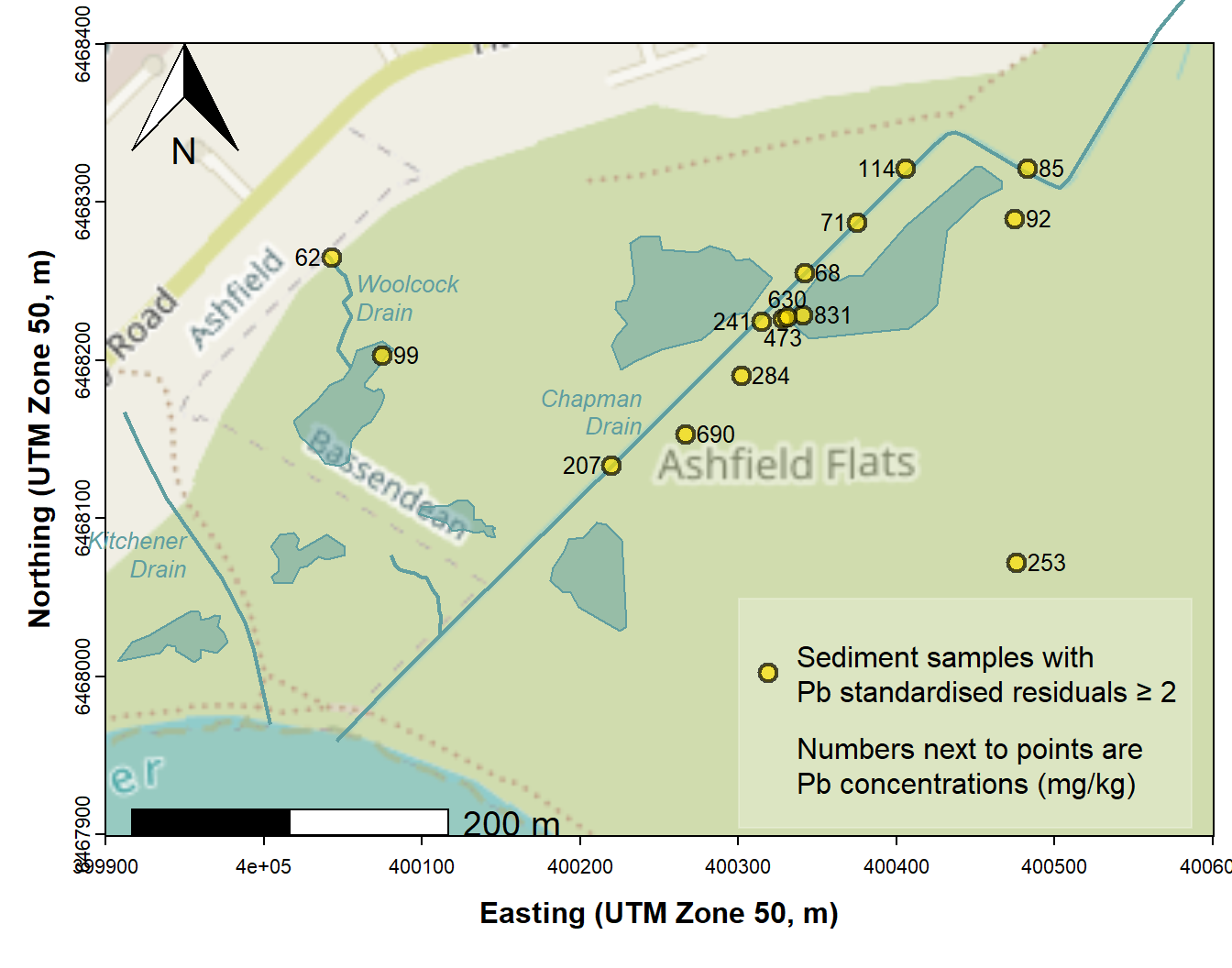
Figure 4: Map of Ashfield Flats showing locations of samples having unusually large Pb concentrations based on a multiple regression model representing a 'background concentration function'.
We should note that the locations identified in Figure 4 do not all
have Pb concentrations greater than the upper guideline value
(GV-high =220 mg/kg), although all have Pb concentrations greater than
the default guideline value (DGV = 50 mg/kg; Water Quality Australia,
2024). Unusual samples with lower Pb concentrations are those which our
model predicts should have a lower background concentration. Based on
the coefficients for each predictor in our model, this means sediments
with low pH, low Al, high Ca, high Fe, low P and high Na. We can
visualise this by plotting the effects for individual predictors using
plot(effects::allEffects(lm1)) from the
effects package.
It's interesting to note that the observations we have identified as unusual, on the basis of having scaled residuals > 2, are also those which are have greater log10Pb concentration greater than the upper bound of the 95% prediction interval for the regression – see Figure 5 below.
par(mfrow=c(1,1), mgp=c(1.5,0.2,0), tcl=0.25, mar=c(3,3,0.5,0.5), las=1, lend="square", xpd=F)
plot(lm1$model$Pb.log ~ lm1$fitted.values,
     xlab=expression(bold(paste(log[10],"Pb predicted by model"))),
     ylab=expression(bold(paste("Observed ",log[10],"Pb"))),
     pch=19, cex=1.2, col="#0000ff40"); abline(0,1,col="sienna")
newdata <- data.frame(pH=seq(min(regdata$pH),max(regdata$pH),l=50),
                      Al=seq(min(regdata$Al),max(regdata$Al),l=50),
                      Ca.log=seq(min(regdata$Ca.log),max(regdata$Ca.log),l=50),
                      Fe=seq(min(regdata$Fe),max(regdata$Fe),l=50),
                      P.log=seq(min(regdata$P.log),max(regdata$P.log),l=50),
                      Na.log=seq(min(regdata$Na.log),max(regdata$Na.log),l=50))
conffit <- predict(lm1, interval = "prediction", level=0.95)
conf0 <- conffit[order(conffit[,1]),]
lines(conf0[,1], conf0[,2], col="grey", lty=3, lwd=2)
lines(conf0[,1], conf0[,3], col="grey", lty=3, lwd=2)
# overplot unusual points separately
hipts <- which(scale(lm1$residuals)>2)
points(lm1$model$Pb.log[hipts] ~ lm1$fitted.values[hipts], pch=22, bg="gold", cex=1.2)
legend("topleft", box.col="grey", inset=c(0.03,0.02), pt.cex=1.2, pch=c(19,22,NA,NA),
       legend=c("Observations","Obs. with scaled residuals > 2","1:1 line","± 95% prediction"),
       col=c("#0000ff40",1,"sienna","grey"), lty=c(NA,NA,1,3),lwd=c(NA,NA,1,2),
       pt.bg=c(NA,"gold",NA,NA), bg="transparent")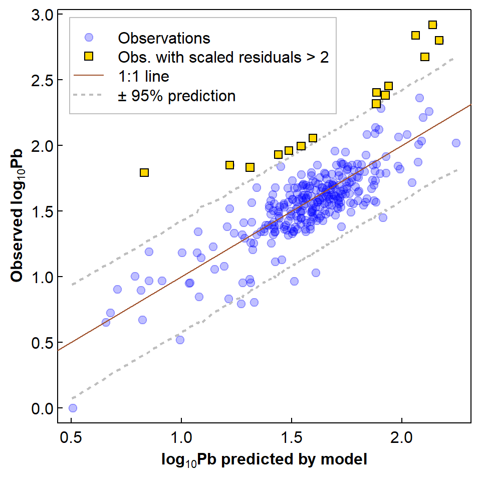
Figure 5: Relationship of observed to predicted log10-Pb showing 1:1 line, 95% prediction interval, and observations with standardised residuals > 2.
The use of regression model residuals to identify unusually high concentrations has made its way into Australian Guidelines for soil contamination (NEPC, 2011). So long as our predictors makes sense in terms of actual biogeochemical controls on contaminant concentrations, this is an approach which would make sense for identifying unusual concentrations for elements which do not yet have guideline values (e.g. Rate, 2018).
References and R packages used
Dunnington, Dewey (2017). prettymapr: Scale Bar,
North Arrow, and Pretty Margins in R. R package version 0.2.2. https://CRAN.R-project.org/package=prettymapr.
Fox J, Weisberg S (2019). An R Companion to
Applied Regression, Third Edition. Thousand Oaks CA: Sage. https://socialsciences.mcmaster.ca/jfox/Books/Companion/
(R packages car and
effects).
Giraud T (2021). maptiles: Download and Display Map
Tiles. R package version 0.3.0, https://CRAN.R-project.org/package=maptiles.
Hamon, R. E., McLaughlin, M. J., Gilkes, R. J., Rate, A. W., Zarcinas, B., Robertson, A., Cozens, G., Radford, N., & Bettenay, L. (2004). Geochemical indices allow estimation of heavy metal background concentrations in soils. Global Biogeochemical Cycles, 18 (GB1014). doi:10.1029/2003GB002063
NEPC (National Environment Protection Council). (2011). Schedule B(1): Guideline on the Investigation Levels for Soil and Groundwater. In National Environment Protection (Assessment of Site Contamination) Measure (Amended). Commonwealth of Australia.
Pebesma, E., 2018. Simple Features for R: Standardized Support for
Spatial VectorData. The R Journal 10 (1),
439-446, doi:10.32614/RJ-2018-009 . (R
package sf)
Rate, A. W. (2018). Multielement geochemistry identifies the spatial pattern of soil and sediment contamination in an urban parkland, Western Australia. Science of The Total Environment, 627, 1106-1120. doi:10.1016/j.scitotenv.2018.01.332
Reimann, C., & Garrett, R. G. (2005). Geochemical background - Concept and reality. Science of The Total Environment, 350, 12-27. doi:10.1016/j.scitotenv.2005.01.047
Water Quality Australia. (2024). Toxicant default guideline values for sediment quality. Department of Climate Change, Energy, the Environment and Water, Government of Australia. Retrieved 2024-04-11 from https://www.waterquality.gov.au/anz-guidelines/guideline-values/default/sediment-quality-toxicants
CC-BY-SA • All content by Ratey-AtUWA. My employer does not necessarily know about or endorse the content of this website.
Created with rmarkdown in RStudio. Currently using the free yeti theme from Bootswatch.