Introduction

Sometimes we can obtain the best map background images in the form of georeferenced images, such as geoTIFF or jpeg. In this example we'll use a jpeg file downloaded from the excellent NearMap site (my university has a subscription 😊). Specialist mapping websites may have better resolution, or have aerial photographs from the most appropriate time of year for our mapping exercise.

First we load the packages that we need:

library(sf)
library(terra)
library(ggplot2)
library(ggspatial)
library(viridis)

We should note that the jpeg file itself doesn't have spatial information, even though we may have downloaded it as a georeferenced image. With jpeg images, georeferencing comes in the form of a companion ('sidecar') file, with the same name but having the .jgw extension. We can read this directly, but the functions we will use below will look for this file and use the spatial information directly. The .jgw file has 6 lines:

length of a pixel in the x direction (horizontal)
angle of rotation (is usually 0 or ignored)
angle of rotation (is usually 0 or ignored)
negative length of a pixel in the y direction (vertical)
x coordinate at centre of pixel in the top left corner of the image
y coordinate at centre of pixel in the top left corner of the image

So long as the file names of the .jpg and .jpw files match, the raster extent and coordinates are obtained or calculated from the values in the .jpw file.

Reading the raster spatial information in the georeferenced jpeg image

We use the terra package, which plays nicely with the sf package, to do most of the work (the sf package was introduced on another page on maps in R. The terra::rast() function will find and use the information in the .jpw file without us specifying that file explicitly.

(AF_nearmap <- 
  terra::rast("EPSG32750_Date20230226_Lat-31.918263_Lon115.944872_Mpp0.597.jpg"))

## class       : SpatRaster
## size        : 795, 1267, 3  (nrow, ncol, nlyr)
## resolution  : 0.597164, 0.597164  (x, y)
## extent      : 399868.4, 400625, 6467901, 6468376  (xmin, xmax, ymin, ymax)
## coord. ref. :
## source      : EPSG32750_Date20230226_Lat-31.918263_Lon115.944872_Mpp0.597.jpg
## colors rgb  : 1, 2, 3
## names       : EPSG32750_~Mpp0.597_1, EPSG32750_~Mpp0.597_2, EPSG32750_~Mpp0.597_3

We notice that, apart from the long and informative filename, the resulting SpatRaster object does not have a coordinate reference system included, so we need to add the appropriate one manually:

terra::crs(AF_nearmap) <- "epsg:32750"
strtrim(st_crs(AF_nearmap),30)

## [1] "WGS 84 / UTM zone 50S"           "PROJCRS[\"WGS 84 / UTM zone 50S"

The messy output above shows that we have what we expect: UTM Zone 50 (south), based on the WGS84 datum.

From the summary of the terra::rast() output above (i.e. colors rgb : 1, 2, 3), we can see that the image has three bands of information, corresponding to the red, green and blue colour channels in the jpeg image.

The object we have created AF_nearmap can be plotted as a map layer.

We need some data to plot, so let's read some:

git <- "https://raw.githubusercontent.com/Ratey-AtUWA/Learn-R-web/refs/heads/main/"
afs1922 <- read.csv(paste0(git,"afs1922edit.csv"), stringsAsFactors = TRUE)
afs1922$Year <- as.factor(afs1922$Year)
(afsREE <- st_as_sf(x = afs1922[,c("Year","Easting", "Northing","Al","Fe","REE")],
         coords = c("Easting", "Northing"), crs = st_crs(32750)))

## Simple feature collection with 262 features and 4 fields
## Geometry type: POINT
## Dimension:     XY
## Bounding box:  xmin: 399908 ymin: 6467930 xmax: 400577 ymax: 6468346
## Projected CRS: WGS 84 / UTM zone 50S
## First 10 features:
##    Year    Al     Fe    REE               geometry
## 1  2019  8996  28836  25.74 POINT (399989 6468038)
## 2  2019 37131  44687 184.71 POINT (399981 6468037)
## 3  2019 28699  48561 161.33 POINT (399971 6468035)
## 4  2019 33882  53061 161.90 POINT (399958 6468028)
## 5  2019 31222  71546 166.20 POINT (399944 6468023)
## 6  2019 34765  38441 142.29 POINT (399930 6468017)
## 7  2019 27926  59783 129.82 POINT (399919 6468014)
## 8  2019 29650  37017 117.57 POINT (399908 6468006)
## 9  2019 17946 135488  71.19 POINT (399971 6468021)
## 10 2019  4114   9255  10.46 POINT (399981 6468052)

We also make a small sf object of the same spatial extent as the background image:

(afrExtent <- 
  st_as_sf(as.data.frame(matrix(st_bbox(AF_nearmap),nrow=2,ncol=2, byrow=T)), 
           coords=c("V1","V2"), crs=32750))

## Simple feature collection with 2 features and 0 fields
## Geometry type: POINT
## Dimension:     XY
## Bounding box:  xmin: 399868.4 ymin: 6467901 xmax: 400625 ymax: 6468376
## Projected CRS: WGS 84 / UTM zone 50S
##                   geometry
## 1 POINT (399868.4 6467901)
## 2   POINT (400625 6468376)

Now we can plot a map with some data on it! We use the image() function to plot the stars raster; we could also use plot() if we specify the argument reset = FALSE.

palette(c("white", mako(8, dir=-1, alpha=0.7), "black","transparent")) # custom palette
par(mar=c(3,3,1,1), oma=c(0,0,0,0), mgp=c(1.6,0.3,0), tcl=-0.2, 
    font.lab=2, cex.lab=1.2, lend="square", ljoin="mitre")
# Plot an empty frame, same size as the stars object
plot(afrExtent$geometry, asp=1, type="n", 
     xaxs="i", yaxs="i",                      # no space around data range
     xlab="Easting (m)", ylab="Northing (m)") 
terra::plot(AF_nearmap, add=TRUE) # add the georeferenced image, and
box()                   # re-draw the box in case of overlap
# plot the points, symbols varying by Year:
#   1. first black unfilled to create 'shadow' behind for better contrast... 
points(st_coordinates(afsREE), pch=c(1,0,5,2)[afsREE$Year], col=10, lwd=2,
       cex=c(1.7,1.6,1.6,1.6)[afsREE$Year])
#   2.  then overplot  with white border. 
points(st_coordinates(afsREE), pch=c(21:24)[afsREE$Year], col=1, lwd=1.5,
       bg=c(2,4,6,8)[afsREE$Year], cex=c(1.5,1.4,1.4,1.4)[afsREE$Year])
# double plot north arrow with small offset to create shadow behind
addnortharrow(pos="topright",padin = c(0.22,0.22), 
              text.col = 10, border = 10, scale=1.4)
addnortharrow(pos="topright",padin = c(0.2,0.2), 
              text.col = 1, border = 1, scale=1.4)
addscalebar(plotepsg=32750, pos="bottomleft",linecol = 1,label.col = 1,
            padin = c(0.22,0.18),htin = 0.2, label.cex = 1.5, widthhint = 0.15)
# add legend for map image and projection information
legend("topleft", title=expression(bold("Ashfield Flats Reserve")),
       legend=c("Photo map source: NearMap Feb 2023 ",
                "EPSG: 32750",
                "(UTM Zone 50 S, WGS84)"),
       box.col="white", bg="#ffffffd0", inset=c(0.01,0.01), 
       title.cex = 1.4, cex=0.9, y.intersp=0.9)
# add legend to identify points by year
legend("bottomright", title=expression(bold("Year")),
       legend=levels(afsREE$Year), text.col = 1, pch=c(21,22,23,24), 
       pt.bg=c(2,4,6,8), col=1, box.col=1, pt.lwd=2, pt.cex=c(1.6,1.4,1.4,1.4), 
       bg = "#707062",inset=c(0.03,0.1), cex=1.2, y.intersp = 1)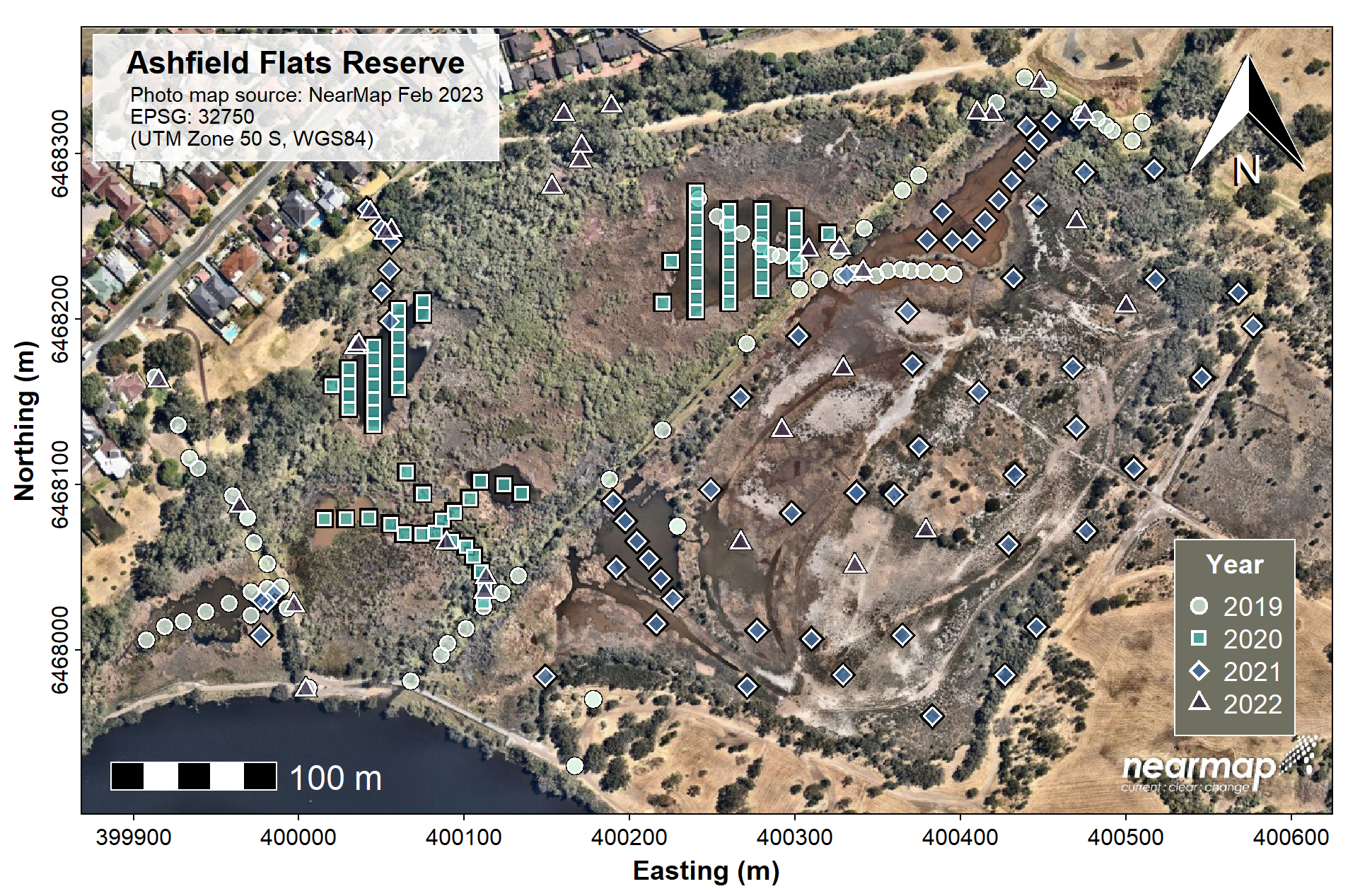

Figure 1: Map of sampling locations at Ashfield Flats Reserve from 2019-2022 plotted on a Nearmap spatial raster.

For comparison we can also use the ggplot2 and ggspatial packages as an alternative...

library(ggplot2)
library(ggspatial)
ggplot() +
  geom_sf(data=afrExtent, col="transparent", fill="transparent") +
  annotation_spatial(data=AF_nearmap) +
  geom_sf(aes(fill=Year, shape=Year), data=afsREE, size=3.5, color="#FFF")+
  annotation_scale(line_col = "#FFF", text_col = "#FFF")+
  annotation_north_arrow(location="tr", 
       style=north_arrow_fancy_orienteering(line_col="#FFF", text_col="#FFF",
                                            text_face="bold")) +
  scale_fill_viridis_d(option="rocket", begin=0.2, end=0.8, alpha=0.8) +
  scale_shape_manual(values=c(21:24))+
  scale_x_continuous(expand=c(0,0)) +
  scale_y_continuous(expand=c(0,0)) +
  labs(x="Longitude",y="Latitude", caption="Aerial photograph from nearmap.com") +
  theme_bw() +
  theme(legend.key = element_rect(fill="#898"),
        axis.title = element_text(face="bold"))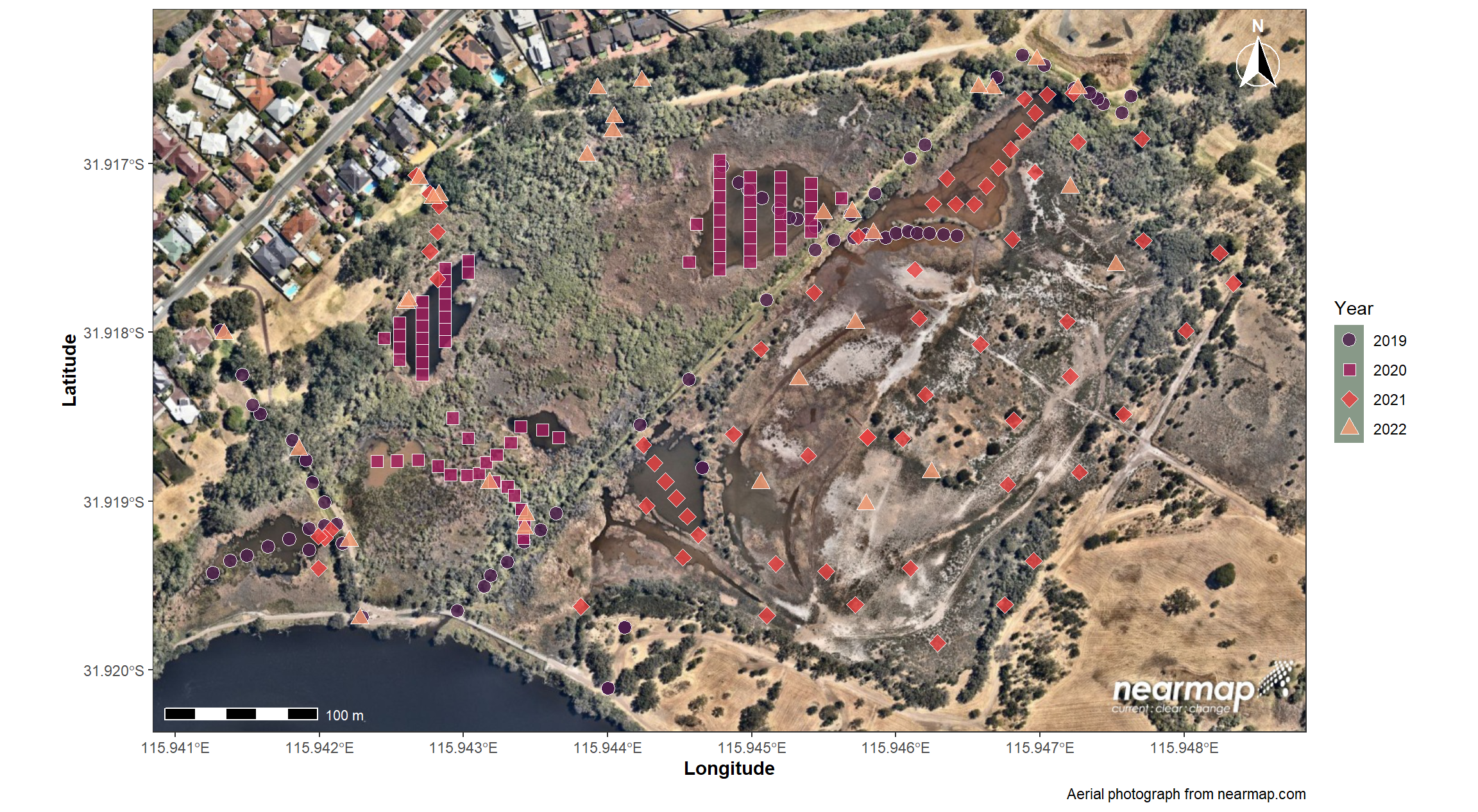

Figure 2: Map of sampling locations at Ashfield Flats Reserve from 2019-2022 plotted on a Nearmap spatial raster using functions from the ggplot2 and ggspatial R packages.

If we include a final line of ggplot code, coord_sf(datum=32750), we can display our axes in UTM (we'd need to change the axis labels).

The choice of plotting package is up to you! We could also add our data in a way that shows values of a variable, as described in the page on maps in R.

Packages

Bivand R, Keitt T, Rowlingson B (2022). rgdal: Bindings for the 'Geospatial' Data Abstraction Library. R package version 1.6-2, https://CRAN.R-project.org/package=rgdal.

Dunnington D (2022). prettymapr: Scale Bar, North Arrow, and Pretty Margins in R. R package version 0.2.4, https://CRAN.R-project.org/package=prettymapr.

Dunnington D (2025). ggspatial: Spatial Data Framework for ggplot2. R package version 1.1.10, doi:10.32614/CRAN.package.ggspatial & https://CRAN.R-project.org/package=ggspatial.

Garnier S., Ross N., Rudis R., Camargo A.P., Sciaini M., and Scherer C. (2021). Rvision - Colorblind-Friendly Color Maps for R. R package version 0.6.2. https://sjmgarnier.github.io/viridis/

Hijmans R, Brown A, Barbosa M (2026). terra: Spatial Data Analysis. R package version 1.9-27, doi:10.32614/CRAN.package.terra.

Pebesma, E., 2018. Simple Features for R: Standardized Support for Spatial Vector Data. The R Journal 10 (1), 439-446, https://doi.org/10.32614/RJ-2018-009

Wickham, H. (2016). ggplot2: Elegant Graphics for Data Analysis. Springer-Verlag, New York https://ggplot2.tidyverse.org

CC-BY-SA • All content by Ratey-AtUWA. My employer does not necessarily know about or endorse the content of this website.
Created with rmarkdown in RStudio. Currently using the free yeti theme from Bootswatch.

Material to support teaching in Environmental Science at The University of Western Australia

Units ENVT3361, ENVT4461, and ENVT5503

Use geotagged jpeg images as map backgrounds

Maps with better aerial photographs

Andrew Rate

2026-09-08

Introduction

Reading the raster spatial information in the georeferenced jpeg image

Packages