Material to support teaching in Environmental Science at The University of Western Australia

Units ENVT3361, ENVT4461, and ENVT5503

Understanding Compositional Data

Compositional data, defined as any measurements which are proportions of some whole, are common in many disciplines, including (Table 1):

Table 1: Examples of compositional data by discipline. All of these examples of data have fixed-sum closure (see below).
Discipline	Examples
Environmental science	Sediment or soil texture - proportions of mineral grains in particle size range fractions
Geography	Proportions of land area subject to different land uses
Geology and geochemistry	Elemental composition of rocks
Biology	Plant species abundance as a proportion of ground cover
Politics	Percentage of voters supporting each candidate

Compositional data have mathematical properties which result in misleading conclusions from traditional statistical analyses. Compositional variables (including concentrations of substances in water [or air, or rock, or soil, and so on] or proportions of land surface coverage) are technically part of a fixed-sum closed set. For example, with data on percent land use over an urban area, all percentages add up to 100%! As Greenacre (2018) points out, we often deal with subcompositions rather than compositions, because we do not (or can not) measure all possible components of a sample. For example, in environmental science, when we measure the substances present in water, we probably can't measure everything, and we don't usually measure the concentration of water itself. Or in politics, we report the proportions of voters who voted for each candidate, but not often the proportion of citizens who didn't vote.

The issue of subcompositions is not necessarily a problem. For instance, in the political example above, the ratio of voters supporting the two leading candidates will be the same whether we consider the total eligible electors, or only the people who actually voted. As we will see below, a key strategy for analysing compositional data is the use of some sort of ratio.

If uncorrected, analysis of data having fixed-sum closure can lead to very misleading conclusions, especially when relationships between variables are being investigated, as in correlation analyses or multivariate methods such as principal component analysis. Closed data require specialised transformations to remove closure, such as calculation of centered or additive log ratios (Reimann et al. 2008). The centered log-ratio is defined by:

\(x_{CLR} = log(\dfrac{x}{geomean(x_{1},...,x_{n})})\), where

\(x\) is the value being transformed (concentration, proportion);
\(x_{CLR}\) is the centered log-ratio transformed value;
\(geomean\) means the geometric mean of;
\(x_{1}...x_{n}\) are all the \(n\) values contributing to the (sub)composition, including the one (\(x\)) being transformed;
all the components (parts) of the composition need to be in identical units (e.g. percent, mg/L, incidence per 10,000, etc.).

For example, in a soil texture analysis where the proportions of grain size categories gravel (G), sand (S), silt (Z), and clay (C) all add up to 100%, the CLR-transformed sand content (S_CLR) is:

\(S_{CLR} = log(\dfrac{S}{geomean(G,S,Z,C)})\)

The example in Figure 1 shows the relationship between phosphorus (P) and iron (Fe) in soil/sediment materials in an acid sulfate environment. Without correcting for compositional closure, the P vs. Fe plot implies that P increases as Fe increases. Correcting for compositional closure, however, suggests the opposite, with P negatively related to Fe! In this case, if we had used conventional transformations, we might have come to a very wrong conclusion about the sediment properties affecting phosphorus.

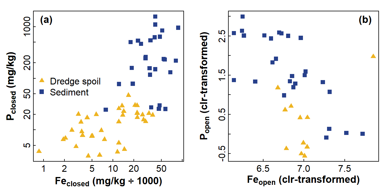
Figure 1: Comparison of relationships between P and Fe for (a) compositionally closed concentrations showing a positive relationship and (b) concentration variables corrected for compositional closure using centred log ratios showing a negative relationship. Data from Xu et al. (2018).

Principal Components Analysis

To get started with understanding compositional data, and analysing them using Principal Components Analysis, we load the packages we need, and set a preferred colour palette.

library(stringr)     # manipulate character strings
library(car)         # statistical functions focused on regression
library(flextable)   # publication-quality tables
library(corrplot)    # correlation heatmaps

palette(c("black", "#003087", "#DAAA00", "#8F92C4", "#E5CF7E", 
          "#001D51", "#B7A99F", "#A51890", "#C5003E", "#FDC596", 
          "#AD5D1E", "gray40", "gray85", "white", "transparent"))

We also need to read some data:

Data are from: Fig. 11 in Hu, J., Wang, Y., Taubenböck, H., Zhu, X.X., 2021. Land consumption in cities: A comparative study across the globe. Cities, 113: 103163, https://doi.org/10.1016/j.cities.2021.103163. (digitised from figure using https://automeris.io/WebPlotDigitizer/)

If you were hoping for an example using geochemical-type compositional data – don't worry, we're going to repeat all the analyses below using a geochemical dataset.

After reading the data we make a column containing abbreviated codes for the land-use type factor, using the gsub() function to substitute character strings.

cities <- 
  read.csv(paste0("https://raw.githubusercontent.com/Ratey-AtUWA/",
                  "compositional_data/main/cities_Hu_etal_2021.csv"), 
           stringsAsFactors = TRUE)
row.names(cities) <- as.character(cities$City)

We also need to use a log-ratio transform to remove compositional fixed-sum closure:

cities_clr <- cities
cities_clr[,2:5] <- t(apply(cities[,2:5], MARGIN = 1,
                           FUN = function(x){log(x) - mean(log(x))}))

Explanation of principal components analysis

It is quite common to measure many variables in environmental science and other disciplines. Using various types of ordination analysis, we can use the information contained in multiple variables to create a reduced subset of variables containing nearly the same amount of information. Ordination methods are also referred to, for this reason, as 'data reduction' methods and are commonly used for multivariate analysis.

One of the earliest and most widely used ordination methods for exploration and dimension-reduction of multivariate data is principal components analysis (PCA). Imagine a dataset with many samples (rows) and n continuous numeric variables (columns) which contain quantitative information about each sample such as concentrations, heights, velocities, etc. For these n variables/dimensions, the principal component calculation generates n new variables, or principal components, which are each a function of the set of all the original variables (so each principal component is defined by a weighting or coefficient for each of the original variables). We may choose to omit some variables from the analysis if they contain too many missing observations or if there is another valid reason to doubt their integrity. Since each principal component is selected to account for successively smaller proportions of the multiple variance, it is usually the first few principal components which explain most of the variance and therefore contain the most useful information. We conventionally visualize this in a 'scree plot' (Figure 2), a kind of bar graph showing the decrease in variance accounted for by each component.

Base-R has two functions which perform Principal Components Analysis (PCA). We will use the prcomp() function which has better numerical accuracy and a more valid variance calculation than the alternative princomp() (see Details after running ?prcomp for more information). We include the argument scale. = TRUE, as this is better for avoiding unexpected results due to large differences in magnitude of the variables.

#
data0 <- na.omit(cities[,c("Compact","Open","Lightweight","Industry")])
pca_cities_clos <- prcomp(data0, scale. = TRUE)
cat("Variable weightings (rotations) - closed data\n")
pca_cities_clos$rot
cat("...\n\nComponent Variances - Closed data\n")
pca_cities_clos$sdev^2
cat("...\n\nProportions of variance explained by each component",
    "\nCLR-transformed (open) data\n")
round(pca_cities_clos$sdev^2/sum(pca_cities_clos$sdev^2),3)
cat("\n--------------------\nVariable weightings (rotations) - open data\n")

data0 <- na.omit(cities_clr[,c("Compact","Open","Lightweight","Industry")])
pca_cities_open <- prcomp(data0, scale. = TRUE)
pca_cities_open$rot
cat("...\n\nComponent Variances - CLR-transformed (open) data\n")
pca_cities_open$sdev^2
cat("...\n\nProportions of variance explained by each component",
    "\nCLR-transformed (open) data\n")
round(pca_cities_open$sdev^2/sum(pca_cities_open$sdev^2),3)
rm(data0)

## Variable weightings (rotations) - closed data
##                    PC1        PC2        PC3         PC4
## Compact     -0.5582052 -0.5356252 0.05639404  0.63113567
## Open        -0.3409659  0.7576682 0.46899761  0.29953715
## Lightweight  0.3992211 -0.3417785 0.85067121 -0.01297763
## Industry    -0.6424731 -0.1491041 0.23069343 -0.71538580
## ...
## 
## Component Variances - Closed data
## [1] 1.5860528 1.0026876 0.8705986 0.5406610
## ...
## 
## Proportions of variance explained by each component 
## CLR-transformed (open) data
## [1] 0.397 0.251 0.218 0.135
## 
## --------------------
## Variable weightings (rotations) - open data
##                    PC1         PC2        PC3        PC4
## Compact     -0.2081793  0.75498116  0.3214239 -0.5323077
## Open        -0.3535490 -0.62668193  0.5577101 -0.4138022
## Lightweight  0.6833728 -0.17189496 -0.2520621 -0.6632635
## Industry    -0.6038759 -0.08789385 -0.7225723 -0.3248042
## ...
## 
## Component Variances - CLR-transformed (open) data
## [1] 1.975945e+00 1.511204e+00 5.128514e-01 1.184394e-31
## ...
## 
## Proportions of variance explained by each component 
## CLR-transformed (open) data
## [1] 0.494 0.378 0.128 0.000

As we should expect, each component accounts for successively less variance. We can already see that removing closure has made a noticeable difference to the PCA output, both in the variable weightings and the component variances.

Principal Components Analysis output

As well as the component variances, the useful results of principal components analysis include the variable weightings or 'rotations' for each principal component. Referring to just the output for open data above, PC1 (which explains the most multivariate variance) has its greatest absolute contributions from the Lightweight and Industry variables, which act in opposite directions (remembering that the sign is arbitrary, but that relative sign and magnitude are important). PC2 contains mainly variance from the Compact and Open variables, PC3 (which explains much less variance) reflects Open/Industry, and we can ignore PC4 as it has a negligible component variance.

In addition, every individual observation (sample) is a multivariate point, the observation scores for all samples in each principal component based on the values of the variables used in PCA for that sample. It is conventional to plot both of these two types of output in a principal component biplot, as shown in Figure 3. Before discussing the biplot, we should note that the sign (positive or negative) of variable weightings and observation scores (i.e. the direction of the axes) is arbitrary and should not affect our interpretations.

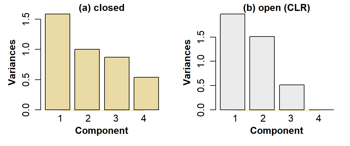
Figure 2: PCA scree plots for urban land-use data, for: (a) compositionally closed proportions; (b) data corrected for closure using CLR-transformation.

There are informal 'rules' for deciding which of the principal components contain useful information:

Components having variance greater than 1 (the 'Kaiser' criterion)
Components up to a cumulative proportion of variance explained of 0.8 (80%)

For example, for the open data, the component variances are PC1 1.976, PC2 1.511, PC3 0.513, PC4 1.5E-31 -- so only PC1 and PC2 meet the first criterion. Similarly, the cumulative proportions of variance explained by each component are PC1 0.494, PC1+PC2 0.872, so by criterion 2 no useful information is contained in principal components >2. In this example both criteria agree (they don't always!).

Another part of the PCA output that we need to know about is the set of observation scores, essentially showing where each observation (each city, in these data) plots in principal component space. We're only interested in PC1 and PC2, since they are the only components meeting the criteria. The observation scores for the first rows of the data are as follows (Table 2):

OScores <- data.frame(City=cities_clr$City[1:8],
                      PC1_closed=round(pca_cities_clos$x[1:8,1],3),
                      PC2_closed=round(pca_cities_clos$x[1:8,2],3),
                      PC1_open=round(pca_cities_open$x[1:8,1],3),
                      PC2_open=round(pca_cities_open$x[1:8,2],3))
flextable(OScores) |>
  theme_zebra(odd_header = "#D0E0FF", even_header = "#D0E0FF") |>
  border_outer(border = BorderDk, part = "all") |>
  border_inner_v(border=BorderLt, part="header") |> 
  set_caption(caption = "Table 2: PCA observation scores for the first 8 rows of the cities data (closed and open).", align_with_table=F, fp_p=fp_par(text.align = "left", padding.bottom = 6))

Table 2: PCA observation scores for the first 8 rows of the cities data (closed and open).
City	PC1_closed	PC2_closed	PC1_open	PC2_open
New York	-1.885	1.095	-0.896	0.155
Sao Paulo	-2.054	-0.732	-0.646	0.722
Shanghai	-2.889	0.909	-1.413	-0.467
Beijing	-1.665	1.230	-0.858	0.098
Jakarta	-2.515	-2.528	-0.592	2.491
Guangzhou	-2.679	-1.453	-1.099	0.957
Melbourne	-1.871	-1.375	-0.808	0.991
Paris	-0.632	2.171	-0.615	-0.489

Principal components biplots

require(car) # for data ellipses (see Fig 1.4)
palette(c("black",scico::scico(8, palette = "batlow", alpha = 0.7),"white"))
par(mfrow=c(1,2), mar = c(3.5,3.5,3.5,3.5), oma = c(0,0,0,0), 
    mgp=c(1.7,0.3,0), tcl = 0.25, font.lab=2,
    lend = "square", ljoin = "mitre")
# choose components and set scaling factor (sf)
v1 <- 1; v2 <- 2; sf <- 0.4

biplot(pca_cities_clos, choices = c(v1,v2), col = c(2,1), cex=c(1,0.0),
       pc.biplot = FALSE, scale = 0.4, arrow.len = 0.08,
       xlim = c(-1.5,1.5), ylim = c(-1.5,1.5),
       xlab = paste0("Scaled PC",v1," Component Loadings"),
       ylab = paste0("Scaled PC",v2," Component Loadings"))
mtext(paste0("Scaled PC",v1," Observation Scores"), 3, 1.6, font = 2)
mtext(paste0("Scaled PC",v2," Observation Scores"), 4, 1.6, font = 2)
mtext("Untransformed data\n(compositionally closed)",
      side = 3, line = -2, font = 2, adj = 0.98)
data0 <- na.omit(cities[,c("Type","Global","Region","Compact",
                           "Open","Lightweight","Industry")])
points(pca_cities_clos$x[,v1]*sf, pca_cities_clos$x[,v2]*sf*1.5,
       pch = c(21:25)[data0$Type],
       lwd = 1, bg = c(7,6,5,4,3)[data0$Type],
       col = 1,
       cex = c(1.4,1.3,1.2,1.2,1.2)[data0$Type])
dataEllipse(x=pca_cities_clos$x[,v1]*sf, y=pca_cities_clos$x[,v2]*sf*1.5,
            groups = data0$Type, add = TRUE, plot.points = FALSE, 
            levels = c(0.9), center.pch = 3, col = c(2,3,8,9,11),
            lty = 2, lwd = 1, center.cex = 2.4, group.labels = "")
legend("bottomright", bty = "o", inset = 0.03,
       box.col = "gray", box.lwd = 2, bg = 10,
       legend = levels(data0$Type),
       pch = c(21:25), pt.lwd = 1,
       col = 1, pt.bg = c(7,6,5,4,3),
       pt.cex = c(1.4, 1.3, 1.2,1.2,1.2),
       cex = 0.9, y.intersp = 0.9)
mtext("(a)", side = 3, line = -1.5, font = 2, adj = 0.02, cex = 1.25)

sf <- 0.25 # adjust scaling factor for next PCA biplot

biplot(pca_cities_open, choices = c(v1,v2), col = c(2,1), cex=c(0.8,1),
       pc.biplot = FALSE, scale = 0.2, arrow.len = 0.08,
       # xlim = c(-1.2,3.2), ylim = c(-3.5,1.7),
       xlab = paste0("Scaled PC",v1," Component Loadings"),
       ylab = paste0("Scaled PC",v2," Component Loadings")) 
mtext(paste0("Scaled PC",v1," Observation Scores"), 3, 1.6, font = 2)
mtext(paste0("Scaled PC",v2," Observation Scores"), 4, 1.6, font = 2)
mtext("CLR\ntransformed\ndata\n(no closure)",
      side = 3, line = -4, font = 2, adj = 0.98)
data0 <- na.omit(cities_clr[,c("Type","Compact","Open","Lightweight","Industry")])
points(pca_cities_open$x[,v1]*sf, pca_cities_open$x[,v2]*sf,
       pch = c(21:25)[data0$Type],
       lwd=2, bg = c(7,6,5,4,3)[data0$Type],
       col = c(1,1,1,1,1)[data0$Type],
       cex = c(1.4,1.3,1.2,1.2,1.2)[data0$Type])
dataEllipse(x=pca_cities_open$x[,v1]*sf, y=pca_cities_open$x[,v2]*sf*1.5,
            groups = data0$Type, add = TRUE, plot.points = FALSE, 
            levels = c(0.9), center.pch = 3, col = c(7,6,5,4,3),
            lty = 2, lwd = 2, center.cex = 2.4, group.labels = "")
legend("bottomright", bty = "o", inset = 0.03,
       box.col = "gray", box.lwd = 2, bg = 10,
       legend = levels(data0$Type),
       pch = c(21:251), pt.lwd = 2,
       col = 1, pt.bg = c(7,6,5,4,3),
       pt.cex = c(1.4, 1.3, 1.2,1.2,1.2),
       cex = 0.9, y.intersp = 0.9)
mtext("(b)", side = 3, line = -1.5, font = 2, adj = 0.02, cex = 1.25)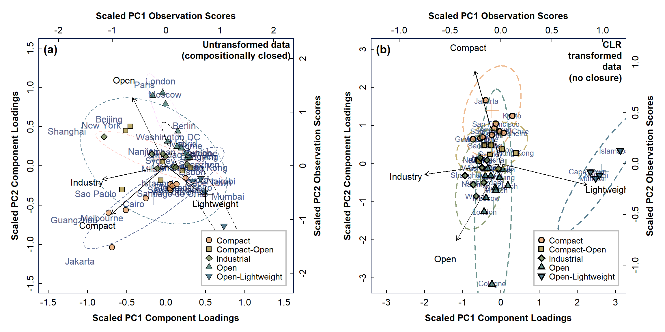

Figure 3: PCA biplots for urban land-use data, with observations categorised by type for: (a) compositionally closed proportions; (b) data corrected for closure using CLR-transformation.

PCA biplots are useful, because the variable weightings group together for variables (measurements) that are related to one another. For example, in the biplots in Figure 3, the variables are relative land areas under 4 land-use categories (which have been corrected in Figure 3(b) for compositional closure using the CLR transformation). These variables are shown as vectors (arrows) in the biplot of principal components PC1 and PC2, and variables which are related have vectors of similar length and/or direction. For example, the variables 'Compact' and 'Industry' plot closely together on biplot (a), suggesting some relationship between these land use categories. Removing closure in our data (biplot (b)) seems to remove this relationship, so it is probably not real!

Often we see the component vectors arranged in an obviously asymmetric pattern with closed data, and this is more apparent further down this page when we analyse some geochemical data. (When closure is removed, the vectors have a less asymmetric pattern - see Figure 5 further below.)

The other main information we obtain from principal components biplots is from the observation scores (see above). These will plot at locations similar to their dominant variables: for example, in Figure 2(b), the 'Compact' cities all plot towards the top of the biplot in the same direction as the 'Compact' variable weighting vector. This suggests that compact cities have greater proportions of compact land use -- which should not be too surprising! Note that in the biplot for closed data in Figure 2(a), the separation of cities is not so clear.

Some other things to try

We could also group the observation scores in our biplot by a different factor in our dataset. For example, it would be interesting to see if we could observe any separation of cities by geographical region in the principal components analysis. You might want to practice your R coding on this problem!

PCA on Geochemical Data

Data edited from: Rate & McGrath (2022a) (described in Rate & McGrath, 2022b).

First we read and curate the data...

ashfield <- 
  read.csv(paste0("https://raw.githubusercontent.com/Ratey-AtUWA/",
                  "compositional_data/main/AFR_surfSed_2019-2021.csv"), 
           stringsAsFactors = TRUE)
ashfield$Year <- as.factor(ashfield$Year)

...and then apply a CLR-transformation to remove closure for the relevant set of variables (i.e. the concentration variables in columns 11:38: Al, As, Ba, Ca, Cd, Ce, Co, Cr, Cu, Fe, Gd, K, La, Li, Mg, Mn, Mo, Na, Nd, Ni, P, Pb, S, Sr, Th, V, Y, Zn.

For the closed data, all elements except Al, Cr, Fe, Gd, K, La, Li, Nd, Ni, Th, V, Y are log₁₀-transformed before PCA to limit the effects of skewness (using scale.=TRUE won't change the shape of variable distributions, unfortunately). We don't remove closure by log₁₀-transformation alone, though.

We also need to make a centered log ratio-transformed dataset.

ashfield_clr <- ashfield
ashfield_clr[,11:38] <- t(apply(ashfield[,11:38], MARGIN = 1,
                                FUN = function(x){log(x) - mean(log(x), na.rm=TRUE)}))
head(ashfield_clr[,11:17])

##         Al        As         Ba       Ca        Cd         Ce        Co
## 1 4.915247 -2.629041 -0.9121439 4.363272 -5.860602 -1.7556753 -0.808294
## 2 5.485119 -3.237030 -0.8175805 3.059425 -5.505493 -0.5044887 -2.056470
## 3 5.453100 -3.673684 -0.8895440 3.585314 -6.701993 -0.4096881 -2.581503
## 4 5.510806        NA -0.3797352 3.032430 -7.305800 -0.5253843 -2.722609
## 5 5.601512 -2.808624 -0.6332189 3.276841 -7.804974 -0.3297310 -2.845259
## 6 5.774326 -3.398333 -0.5061159 3.665076 -8.188598 -0.3984539 -2.680560

Inspect correlation matrix first

par(mfrow=c(1,2), mar=c(5,4,6,2))
corC <- cor(ashfield[,11:38], use="pairwise.complete.obs", method="spearman")
corrplot::corrplot(corC, title="\n(a)", method="ellipse", diag=F, tl.col = 1)
corO <- cor(ashfield_clr[,11:38], use="pairwise.complete.obs", method="spearman")
corrplot::corrplot(corO, title="\n(b)", method="ellipse", diag=F, tl.col = 1)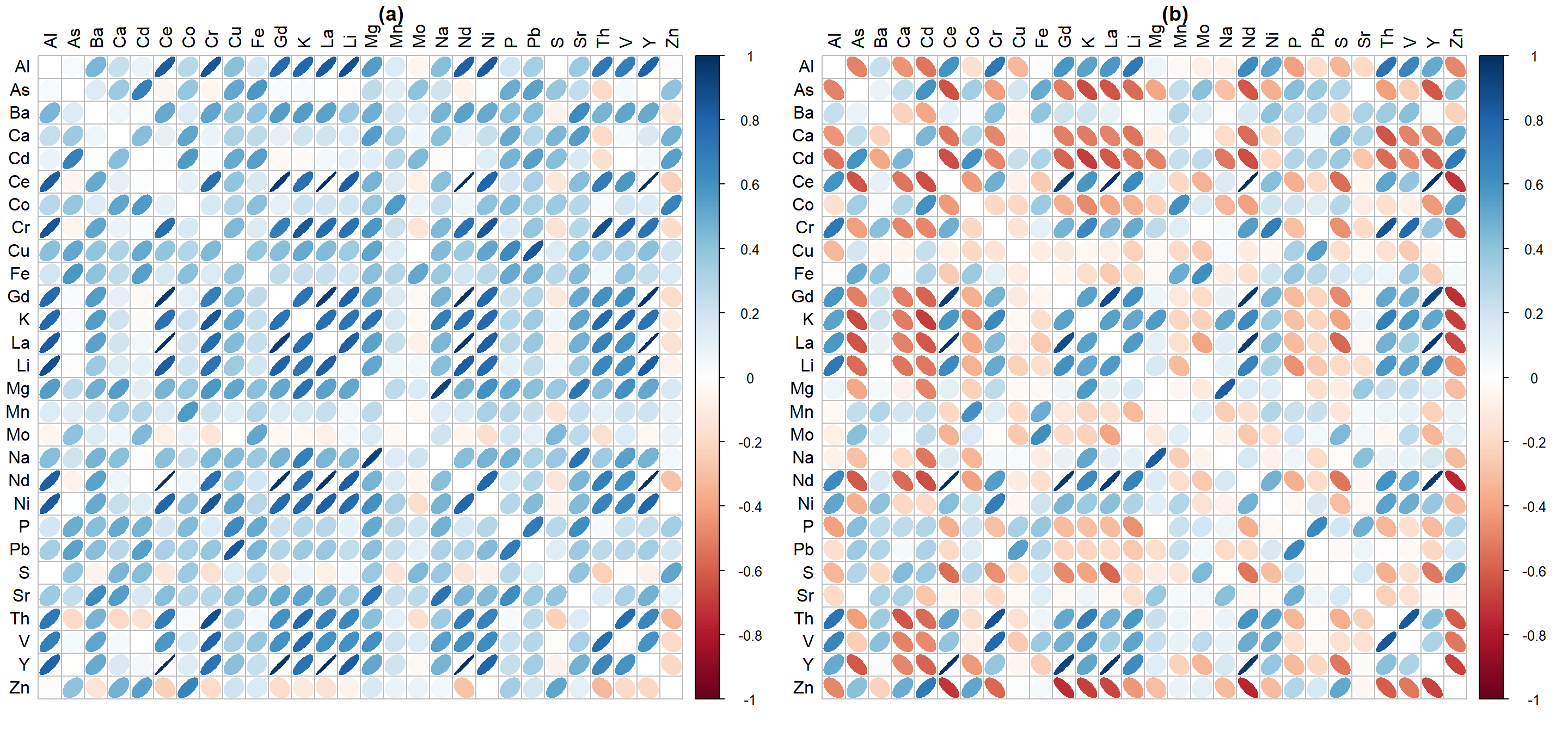

Figure 4: Correlation heatmaps showing relationships based on Spearman correlations between elements in (a) compositionally closed data and (b) clr-transformed 'opened' data (both from Ashfield Flats 2019-2021).

Figure 4 shows that between-element correlations are profoundly different when compositional closure is removed by centered-log-ratio transformation. Strictly speaking, we should always use CLR-transformed concentrations when examining relationships between chemical components of environmental samples.

Running the geochemical PCA

We run the PCA using prcomp() using scale. = TRUE as before, for both closed and CLR-transformed concentrations:

data0 <- na.omit(ashfield[,c(3,4,11:38)])
forlog <- c("As","Ba","Ca","Cd","Ce","Co","Cu","Mg",
            "Mn","Mo","Na","P","Pb","S","Sr","Zn")
data0[,which(colnames(data0) %in% forlog==T)] <- 
  log10(data0[,which(colnames(data0) %in% forlog==T)]) # note log-transformation
pca_ashfield_clos <- prcomp(data0[,3:30], scale. = TRUE)
cat("Variable weightings (rotations) - Closed data (only simple transformations) (first 8 PCs, first 6 variables)\n")
head(pca_ashfield_clos$rot[,1:8])
cat("...\n\nComponent Variances - Closed data (only simple transformations)\n")
pca_ashfield_clos$sdev^2
cat("...\n\nProportions of variance explained by each component",
    "\nClosed data (only simple transformations)\n")
round(pca_ashfield_clos$sdev^2/sum(pca_ashfield_clos$sdev^2),3)
cat("\nCumulative proportions of variance explained by each component",
    "\nClosed data (only simple transformations)\n")
cumsum(round(pca_ashfield_clos$sdev^2/sum(pca_ashfield_clos$sdev^2),3))

cat("\n--------------------\nVariable weightings (rotations) - open data (first 8 PCs, first 6 variables)\n")
data0 <- na.omit(ashfield_clr[,c(3,4,11:38)])
pca_ashfield_open <- prcomp(data0[,3:30], scale. = TRUE)
head(pca_ashfield_open$rot[,1:8])
cat("...\n\nComponent Variances - CLR-transformed (open) data\n")
pca_ashfield_open$sdev^2
cat("...\n\nProportions of variance explained by each component",
    "\nCLR-transformed (open) data\n")
round(pca_ashfield_open$sdev^2/sum(pca_ashfield_open$sdev^2),3)
cat("\nCumulative proportions of variance explained by each component",
    "\nCLR-transformed (open) data\n")
cumsum(round(pca_ashfield_open$sdev^2/sum(pca_ashfield_open$sdev^2),3))

## Variable weightings (rotations) - Closed data (only simple transformations) (first 8 PCs, first 6 variables)
##             PC1          PC2         PC3         PC4         PC5         PC6
## Al  0.262841876  0.017144343 -0.03340468  0.07557376 -0.02000568  0.12582389
## As -0.008274958 -0.318481074  0.32606705 -0.15555049  0.04373040  0.08520550
## Ba  0.223649632 -0.008918856  0.10460779 -0.02859546 -0.02721085 -0.07730027
## Ca -0.003890032 -0.270074999 -0.22805374  0.31810269  0.17176970 -0.23038375
## Cd -0.007462965 -0.353406876  0.09916246  0.04792640 -0.13819598  0.26012265
## Ce  0.270588496  0.055330381  0.03351360  0.04960608  0.11573493  0.07281675
##            PC7         PC8
## Al -0.14426303  0.01632898
## As  0.07421221  0.11276656
## Ba  0.09108350  0.69439959
## Ca  0.16281311  0.02894780
## Cd -0.09793862 -0.21727179
## Ce  0.08373182 -0.05420771
## ...
## 
## Component Variances - Closed data (only simple transformations)
##  [1] 12.032835073  5.299682267  2.008113141  1.707073819  1.410281801  1.208587356
##  [7]  0.871576056  0.536311687  0.495569067  0.452154244  0.344878927  0.311959327
## [13]  0.225668949  0.189165871  0.157172071  0.140098666  0.132463354  0.111278485
## [19]  0.085343162  0.079540396  0.055650771  0.039918372  0.031313004  0.029117363
## [25]  0.021903268  0.016070376  0.004875592  0.001397537
## ...
## 
## Proportions of variance explained by each component 
## Closed data (only simple transformations)
##  [1] 0.430 0.189 0.072 0.061 0.050 0.043 0.031 0.019 0.018 0.016 0.012 0.011 0.008
## [14] 0.007 0.006 0.005 0.005 0.004 0.003 0.003 0.002 0.001 0.001 0.001 0.001 0.001
## [27] 0.000 0.000
## 
## Cumulative proportions of variance explained by each component 
## Closed data (only simple transformations)
##  [1] 0.430 0.619 0.691 0.752 0.802 0.845 0.876 0.895 0.913 0.929 0.941 0.952 0.960
## [14] 0.967 0.973 0.978 0.983 0.987 0.990 0.993 0.995 0.996 0.997 0.998 0.999 1.000
## [27] 1.000 1.000
## 
## --------------------
## Variable weightings (rotations) - open data (first 8 PCs, first 6 variables)
##           PC1          PC2          PC3         PC4         PC5         PC6
## Al  0.2178761 -0.175508744  0.110495240 -0.06970021  0.07015334 -0.02101289
## As -0.2047095 -0.181257338 -0.202507482  0.10924893  0.10719031 -0.11524954
## Ba  0.1050193 -0.150214445 -0.047486395 -0.02175757 -0.14850985 -0.61186474
## Ca -0.1738396  0.045453704  0.199087874 -0.28077341 -0.06087187 -0.18134128
## Cd -0.2318630 -0.144853181  0.008502368  0.02861680  0.07265346  0.22920487
## Ce  0.2627008 -0.002588997 -0.144448507 -0.17814957  0.16699334  0.04285596
##            PC7        PC8
## Al  0.20442617 -0.1993189
## As -0.08703576 -0.2380530
## Ba  0.39012320  0.4123293
## Ca -0.09351070 -0.5848205
## Cd -0.04565633  0.2309725
## Ce -0.05901182  0.0236751
## ...
## 
## Component Variances - CLR-transformed (open) data
##  [1] 1.165706e+01 3.619179e+00 2.753411e+00 2.339868e+00 1.638357e+00 1.240181e+00
##  [7] 8.625783e-01 6.309300e-01 5.935636e-01 4.648664e-01 4.266296e-01 2.947315e-01
## [13] 2.784008e-01 2.291795e-01 1.888286e-01 1.552614e-01 1.497596e-01 1.258552e-01
## [19] 9.168352e-02 7.637244e-02 5.451782e-02 3.796124e-02 3.090203e-02 2.757347e-02
## [25] 2.237504e-02 8.676022e-03 1.298201e-03 3.105273e-30
## ...
## 
## Proportions of variance explained by each component 
## CLR-transformed (open) data
##  [1] 0.416 0.129 0.098 0.084 0.059 0.044 0.031 0.023 0.021 0.017 0.015 0.011 0.010
## [14] 0.008 0.007 0.006 0.005 0.004 0.003 0.003 0.002 0.001 0.001 0.001 0.001 0.000
## [27] 0.000 0.000
## 
## Cumulative proportions of variance explained by each component 
## CLR-transformed (open) data
##  [1] 0.416 0.545 0.643 0.727 0.786 0.830 0.861 0.884 0.905 0.922 0.937 0.948 0.958
## [14] 0.966 0.973 0.979 0.984 0.988 0.991 0.994 0.996 0.997 0.998 0.999 1.000 1.000
## [27] 1.000 1.000

For both the closed and open data, we reach 80% of variance explained by component 6.

Figure 5: PCA scree plots for Ashfield data, for: (a) compositionally closed concentrations (only simple transformations); (b) data corrected for closure using CLR-transformation.

Figure 5 shows that for this analysis, 6 components have variances ≥ 1, regardless of closure.

OScores <- data.frame(Samp=ashfield_clr$SampID[1:8],
                      PC1_closed=round(pca_ashfield_clos$x[1:8,1],3),
                      PC2_closed=round(pca_ashfield_clos$x[1:8,2],3),
                      PC1_open=round(pca_ashfield_open$x[1:8,1],3),
                      PC2_open=round(pca_ashfield_open$x[1:8,2],3))
flextable(OScores) |>
  theme_zebra(odd_header = "#D0E0FF", even_header = "#D0E0FF") |>
  border_outer(border = BorderDk, part = "all") |>
  border_inner_v(border=BorderLt, part="header") |>
  set_caption(caption="Table 3: PCA observation scores for the first 8 rows of the Ashfield Flats data (closed and open).", align_with_table=F, fp_p=fp_par(text.align = "left", padding.bottom = 6))

Table 3: PCA observation scores for the first 8 rows of the Ashfield Flats data (closed and open).
Samp	PC1_closed	PC2_closed	PC1_open	PC2_open
2019_1_1	-5.146	-2.714	-7.490	4.090
2019_1_2	2.327	-1.885	-0.544	1.529
2019_1_3	1.030	-0.447	0.637	2.714
2019_1_4	1.426	-0.136	1.237	1.460
2019_1_5	1.105	0.705	1.819	2.410
2019_1_6	0.982	-0.781	0.087	2.629
2019_1_7	0.391	0.176	0.877	3.000
2019_1_8	-0.489	-3.817	-3.505	2.875

par(mfrow=c(1,2), mar = c(3.5,3.5,3.5,3.5), oma = c(0,0,0,0), 
    mgp=c(1.7,0.3,0), tcl = 0.25, font.lab=2,
    lend = "square", ljoin = "mitre")
# choose components and set scaling factor (s0)
v1 <- 1; v2 <- 2; s0 <- 0.12

biplot(pca_ashfield_clos, choices = c(v1,v2), col = c("#ffffff00",1), cex=c(1,0.0),
       pc.biplot = FALSE, scale = 0.4, arrow.len = 0.08,
       # xlim = c(-1.5,1.5), ylim = c(-1.2,1.2),
       xlab = paste0("Scaled PC",v1," Component Loadings"),
       ylab = paste0("Scaled PC",v2," Component Loadings"))
mtext(paste0("Scaled PC",v1," Observation Scores"), 3, 1.6, font = 2)
mtext(paste0("Scaled PC",v2," Observation Scores"), 4, 1.6, font = 2)
mtext("Untransformed data\n(compositionally closed)",
      side = 1, line = -2, font = 2, adj = 0.04)
data0 <- na.omit(ashfield[,c(3,4,9:38)])
points(pca_ashfield_clos$x[,v1]*s0, pca_ashfield_clos$x[,v2]*s0*1.5,
       pch = c(22,21,24)[data0$Type],
       lwd = 1, bg = c(6,4,2)[data0$Type],
       col = 1,
       cex = c(1.2,1.4,1)[data0$Type])
legend("bottomright", bty = "o", inset = 0.03,
       box.col = "gray", box.lwd = 2, bg = 10,
       legend = levels(data0$Type),
       pch = c(22,21,24), pt.lwd = 1
       ,
       col = 1, pt.bg = c(6,4,2),
       pt.cex = c(1.2, 1.4, 1),
       cex = 0.9, y.intersp = 0.9)
mtext("(a)", side = 3, line = -1.5, font = 2, adj = 0.02, cex = 1.25)

s0 <- 0.09 # adjust scaling factor for next PCA biplot

biplot(pca_ashfield_open, choices = c(v1,v2), col = c("transparent",1), cex=c(0.8,1),
       pc.biplot = FALSE, scale = 0.2, arrow.len = 0.08,
       # xlim = c(-1.2,3.2), ylim = c(-3.5,1.7),
       xlab = paste0("Scaled PC",v1," Component Loadings"),
       ylab = paste0("Scaled PC",v2," Component Loadings")) 
mtext(paste0("Scaled PC",v1," Observation Scores"), 3, 1.6, font = 2)
mtext(paste0("Scaled PC",v2," Observation Scores"), 4, 1.6, font = 2)
mtext("CLR-transformed\ndata (no closure)",
      side = 1, line = -2, font = 2, adj = 0.04)
data0 <- na.omit(ashfield_clr[,c(3,4,9:38)])
points(pca_ashfield_open$x[,v1]*s0, pca_ashfield_open$x[,v2]*s0,
       pch = c(22,21,24)[data0$Type],
       lwd = 1, bg = c(6,4,2)[data0$Type],
       col = 1,
       cex = c(1.2,1.4,1)[data0$Type])
legend("bottomright", bty = "o", inset = 0.03,
       box.col = "gray", box.lwd = 2, bg = 10,
       legend = levels(data0$Type),
       pch = c(22,21,24), pt.lwd = 1,
       col = 1, pt.bg = c(6,4,2),
       pt.cex = c(1.2, 1.4, 1),
       cex = 0.9, y.intersp = 0.9)
mtext("(b)", side = 3, line = -1.5, font = 2, adj = 0.02, cex = 1.25)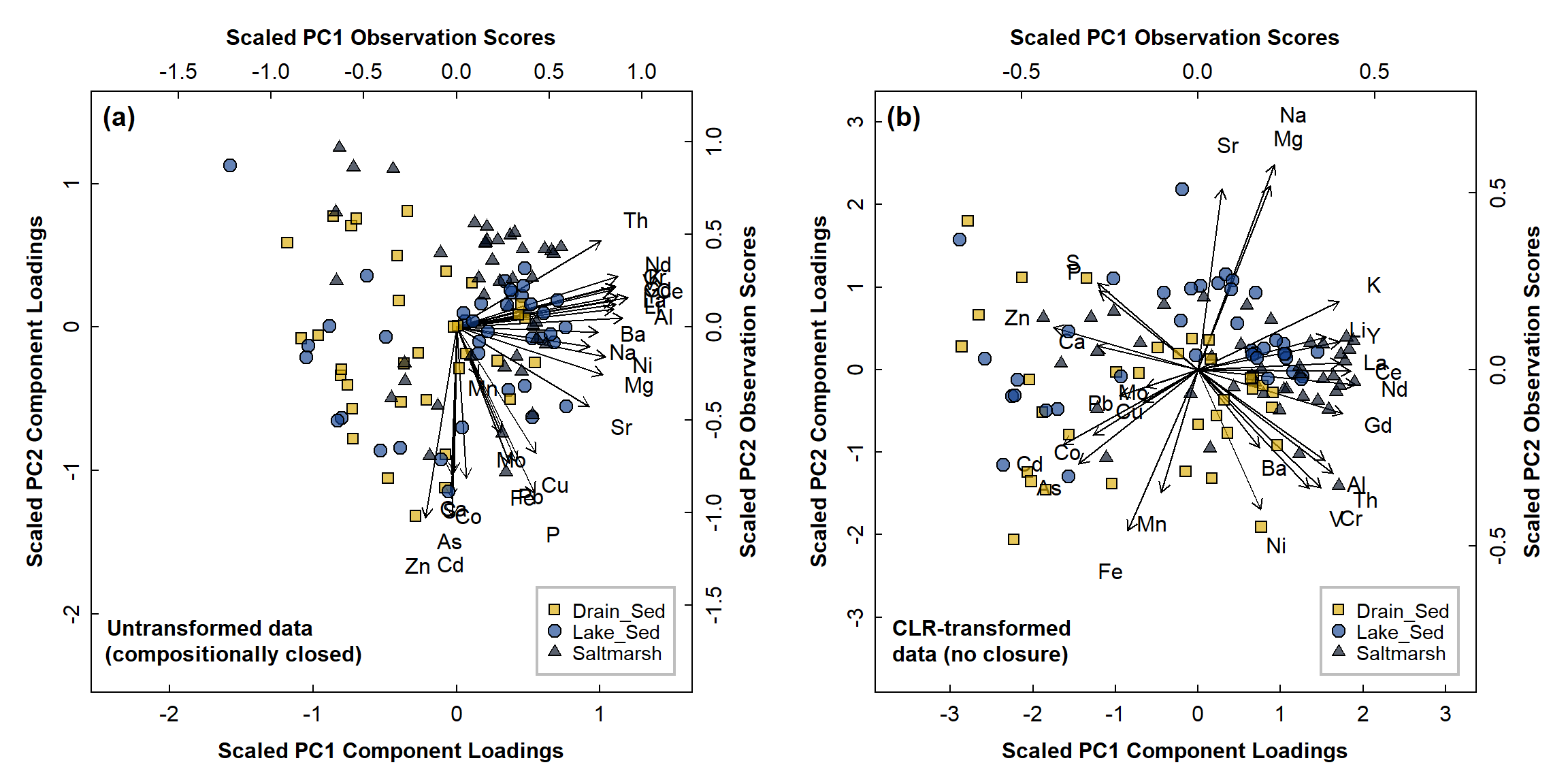

Figure 6: PCA biplots for Ashfield data, with observations categorised by sample type for: (a) compositionally closed concentrations, log~10~ transformation only; (b) data corrected for closure using CLR-transformation.

Figure 6: PCA biplots for Ashfield data, with observations categorised by sample type for: (a) compositionally closed concentrations, log₁₀ transformation only; (b) data corrected for closure using CLR-transformation.

We can see some interesting effects in Figure 6:

there is obvious asymmetry in the biplot for the closed data (Figure 6(a)) which can make any effects hard to interpret, even if they were valid
in the biplot for open (clr-transformed) data (Figure 6(b)), some of the elemental associations make sense (e.g. Sr-Na-Mg, the REEs Ce-La-Nd-Gd-(Y), Al with Cr, Th, and V (and possibly REEs), redox-sensitive elements Fe-Mn, etc.)
some clustering of observations is apparent in Figure 6(b), e.g. some Saltmarsh sediments seem to be associated with high REE concentrations; drain sediments are mainly towards the lower left
- we may see clearer clustering by plotting different pairs of principal components, e.g. PC1 vs. PC3, PC2 vs. PC3. Remember from above that six principal component dimensions possibly contain useful information.
- also, the PCA procedure maximises multiple variance, not the separation between groups. There are other multivariate methods that can do that, like discriminant analysis.

We might see clearer groupings based on a different factor, such as whether the sample location has a tidal influence or not, or a finer categorisation by individual wetland pond.

The PCA output should extend the information we get from a correlation matrix (Figure 7). The PCA biplot in Figure 6(b) suggests several groups of correlated elements which is reinforced by Figure 7. For example, the rare earth elements Ce, Gd, La, and Nd are all positively correlated, and their association is also shown in the PCA biplot by the vectors (arrows) for Ce, Gd, La, and Nd pointing in very similar directions. Conversely, there is a significant negative correlation between Cr and Zn, which is shown on the PCA biplot by the Cr and Zn vectors pointing in nearly opposite directions.

The PCA biplot does more than just enhance the correlation matrix, however. We also plot the observations (i.e. samples) on the biplot. We can see, for example, that samples close to the Ce, Gd, La, and Nd vectors are mainly saltmarsh and lake sediments, and so we assume that Ce, Gd, La, and Nd concentrations are greater in these environments. (We could also express this by stating that “saltmarsh and lake sediments are characterised by greater concentrations of Ce, Gd, La, and Nd”).

library(psych) ; library(corrplot)
par(family="nar")
data0 <- na.omit(ashfield_clr[,c("pH","Al","Ca","Fe","As","Cd","Cr",
                                 "Cu","Mn","Na","Ni","P","Pb","S",
                                 "Sr","Zn","Ce","Gd","La","Nd")])
cormat <- corTest(data0)
corPvals <- cormat$p
corPvals[upper.tri(corPvals)] <- cormat$p.adj
corPvals <- t(corPvals)
corPvals[upper.tri(corPvals)] <- cormat$p.adj
corPvals <- t(corPvals)
corrplot(cormat$r, method="ellipse", type="upper", diag=F, 
         tl.col=1, tl.pos="t", mar=c(3,2,1,1), cl.cex=1.4, 
         tl.cex=1.4)
corrplot(cormat$r, method="square", type="lower", diag=F, 
         tl.col=1, tl.pos="l", tl.cex=1.4, addCoef.col="black", 
         number.cex=1., add=T, p.mat=corPvals, is.corr=F, 
         insig = "pch", pch=15, pch.col="#ffffffe0", pch.cex = 5, 
         addCoefasPercent=F, cl.pos="n",
         col=colorRampPalette(c("tomato","white","steelblue"))(128))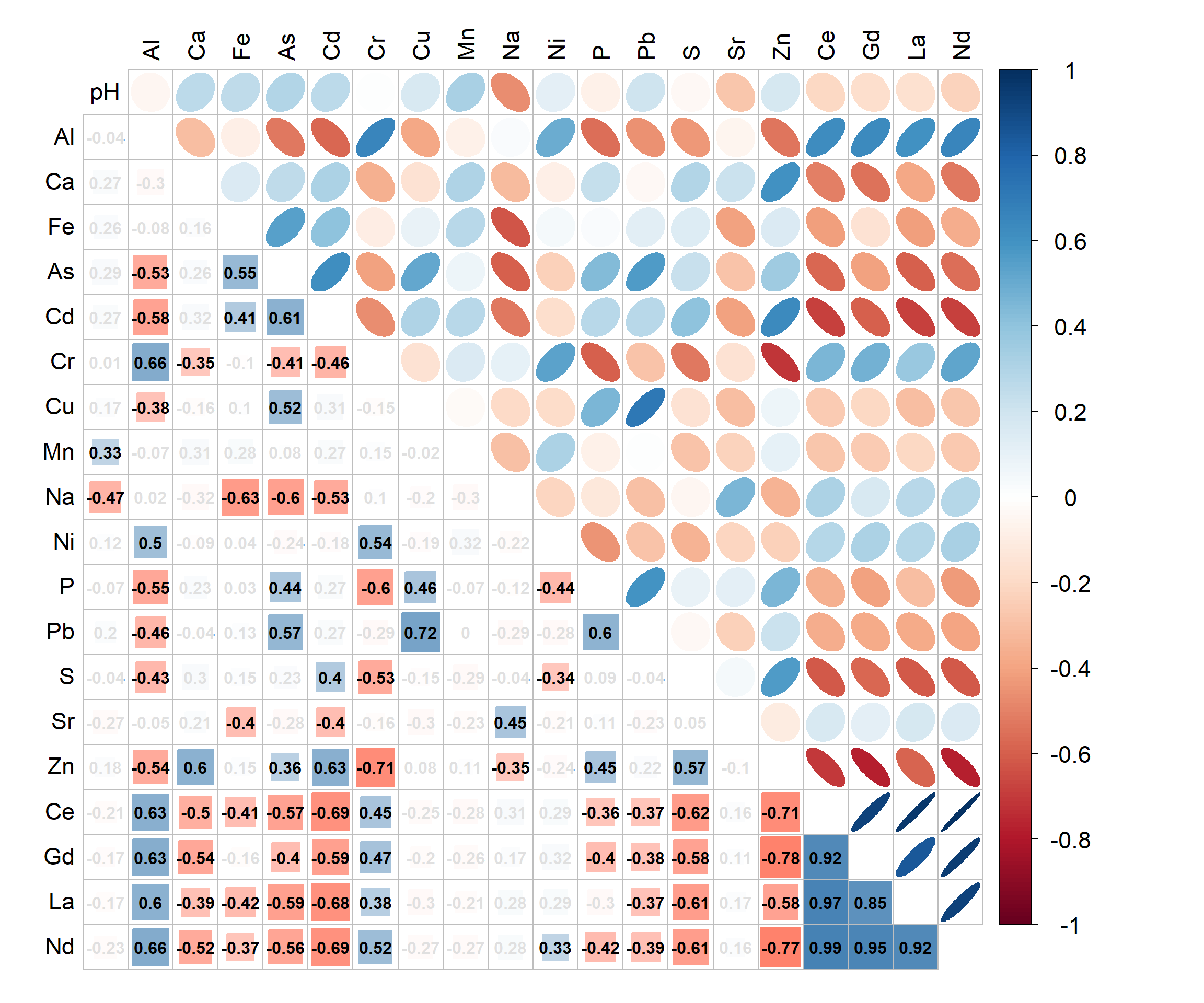

Figure 7: Correlation matrix and heatmap for concentrations of selected elements in sediments from Ashfield Flats 2019-2021. Lower triangle of correlation matrix shows Pearson's r values with non-significant correlations (Holm's adjusted p > 0.05) ‘greyed-out’.

Let's have a look at plotting other PCA dimensions (just for the clr-transformed data, since that's the correct way to do it). The output of the code below is in Figure 8.

data0 <- na.omit(ashfield_clr[,c(3,4,11:38)])
palette(c("black","moccasin","cyan2","navy","gray33"))
par(mfrow=c(3,2), mar = c(3,3,3,3), oma = c(0,0,0,0), 
    mgp=c(1.3,0.2,0), tcl = 0.25, font.lab=2, cex.lab=1.2,
    lend = "square", ljoin = "mitre")
v1list <- c(1,1,2,2,3) ; v2list <- c(3,4,3,4,4)
s0 <- 0.09 # components & scaling factor for this plot
for(i in 1:5){
  v1 <- v1list[i]; v2 <- v2list[i]; s0s <- c(0.09,0.12,0.14,0.12,0.14)
  biplot(pca_ashfield_open, choices = c(v1,v2), col = c("transparent",5), cex=c(0.8,1),
         pc.biplot = FALSE, scale = 0.2, arrow.len = 0.08,
         # xlim = c(-1.2,3.2), ylim = c(-3.5,1.7),
         xlab = paste0("Scaled PC",v1," Component Loadings"),
         ylab = paste0("Scaled PC",v2," Component Loadings")) 
  mtext(paste0("Scaled PC",v1," Observation Scores"), 3, 1.3, font = 2, cex=0.8)
  mtext(paste0("Scaled PC",v2," Observation Scores"), 4, 1.3, font = 2, cex=0.8)
  points(pca_ashfield_open$x[,v1]*s0s[i], pca_ashfield_open$x[,v2]*s0s[i],
         pch = c(22,21,24)[data0$Type],
         lwd = 1, bg = c(2,3,4)[data0$Type],
         col = 1,
         cex = c(1.2,1.4,1)[data0$Type])
  mtext(paste0("(",letters[i],") PC",v2," vs. PC",v1), 
        side = 3, line = -1.5, font = 2, adj = 0.02)
}
plot(0:1,0:1, type="n",bty="n",axes=F,ann=F)
legend("topleft", bty = "o", inset = 0.03,
        box.col = "gray", box.lwd = 2, bg = "white",
        legend = levels(data0$Type), title="Sample Type",
         pch = c(22,21,24), pt.lwd = 1,
         col = 1, pt.bg = c(2,3,4),
         pt.cex = c(1.2, 1.4, 1)*1.4,
         cex = 1.4, y.intersp = 0.9)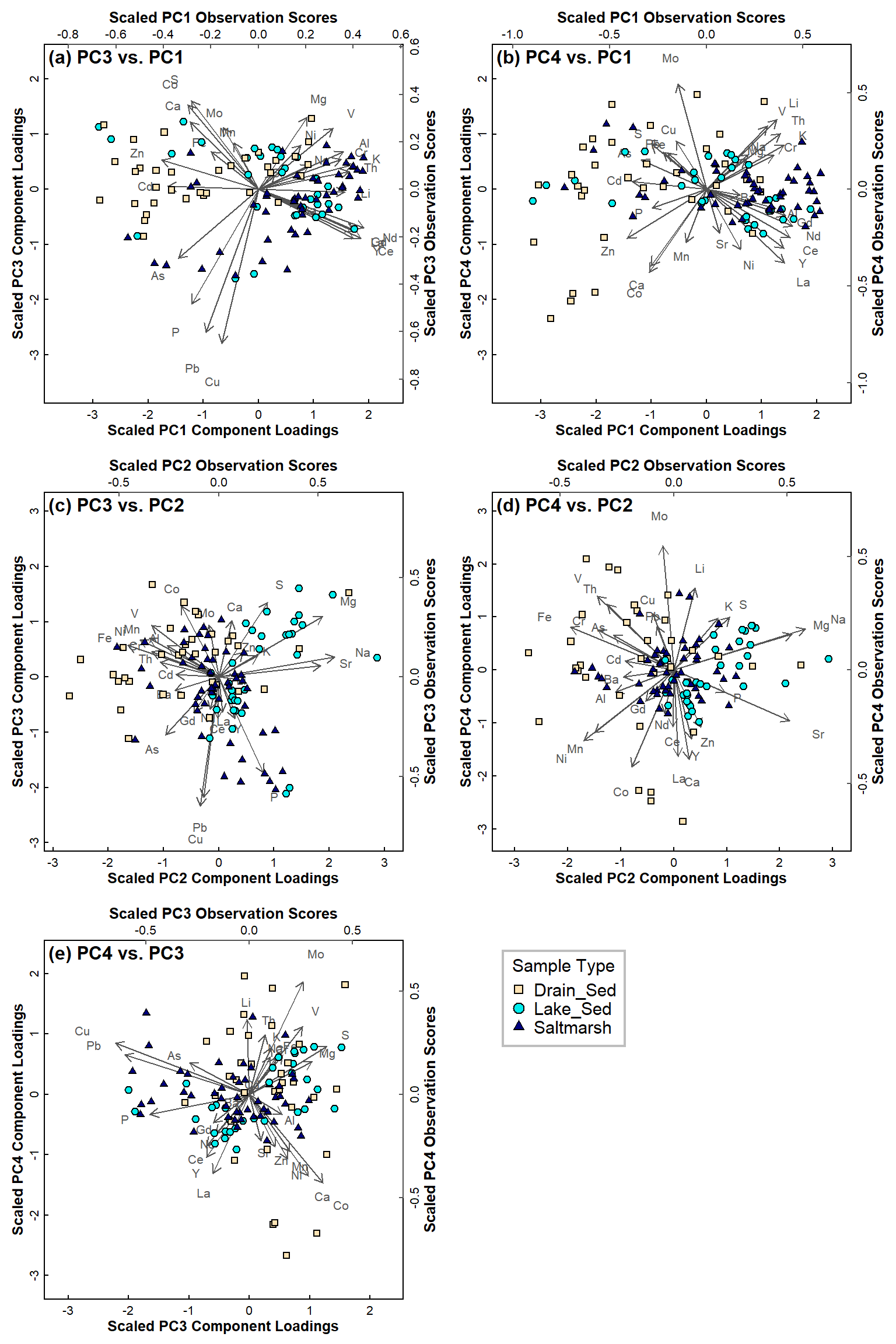

Figure 8: PCA biplots for Ashfield data, with observations categorised by sample type for: (a) PC3 vs. PC1; (b) PC4 vs. PC1; (c) PC3 vs. PC2; (d) PC4 vs. PC2; (e) PC4 vs. PC3.

The higher-order principal components do not add that much to the information we get from PC1 and PC2 in Figure 6. This is expected, since the first two principal components explain about 55% of the multiple variance. The PC3~PC1 and PC4~PC1 biplots suggest that Drain sediments have greater Zn than sediments from other areas.

Alternatively we could look at a 3D plot (Figure 9) using the scatterplot3d package.

library(scatterplot3d)
data0 <- na.omit(ashfield_clr[,c(3,4,11:38)])
palette(c("black",colorRampPalette(c("navy","cyan2","moccasin"))(7),
          "grey","#ffffffa0"))
par(mfrow=c(1,2), mgp=c(1.6,0.2,0), font.lab=2)
s3d <- scatterplot3d(x=pca_ashfield_open$x[,1], 
                     y=pca_ashfield_open$x[,2], 
                     z=pca_ashfield_open$x[,3], mar=c(3,3,1,2.6),
              box=T, grid=T, type="p", col.axis="grey", angle=25, scale.y = 0.8, 
              bg = c(2,5,8)[data0$Type], 
              pch = c(21,22,23)[data0$Type], main="(a)",
              xlab="PC1 observation score", ylab="PC2 observation score",zlab="PC3 observation score")
legend(s3d$xyz.convert(-11, 0, -4), legend = levels(data0$Type),
      title="Sample Type", pt.bg= c(2,5,8), pch=c(21,22,23), box.col=10, bg=10)
s3d <- scatterplot3d(x=pca_ashfield_open$rotation[,1], 
                     y=pca_ashfield_open$rotation[,2], 
                     z=pca_ashfield_open$rotation[,3], mar=c(3,3,1,2.6),
                     box=T, grid=T, type="p", col.axis="grey", angle=25, scale.y = 0.75, 
                     pch = 1, cex.symbols=3, color="gray", main="(b)",
                     xlab="PC1 Variable Rotation", ylab="PC2 Variable Rotation",zlab="PC3 Variable Rotation")
text(s3d$xyz.convert(pca_ashfield_open$rotation[, 1:3]), labels = rownames(pca_ashfield_open$rotation),
     cex= 0.85)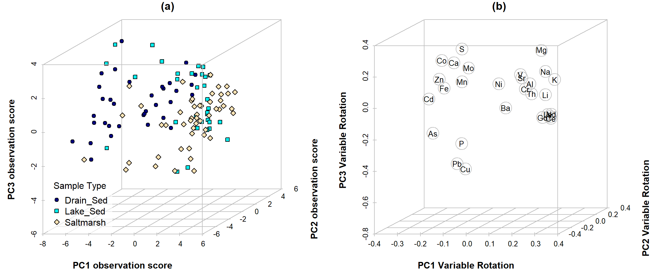

Figure 9: Plot of (a) observation scores and (b) component (variable) loadings for PCA on clr-transformed sediment elemental concentrations from Ashfield Flats 2019-2021.

References and R Packages

Fox, J. (2022). RcmdrMisc: R Commander Miscellaneous Functions. R package version 2.7-2. https://CRAN.R-project.org/package=RcmdrMisc

John Fox and Sanford Weisberg (2019). An {R} Companion to Applied Regression (car), Third Edition. Thousand Oaks CA: Sage. URL: https://socialsciences.mcmaster.ca/jfox/Books/Companion/

Greenacre, M. (2018). Compositional Data Analysis in Practice. CRC Press LLC, Boca Raton, FL, USA.

Hu, J., Wang, Y., Taubenböck, H., Zhu, X.X. (2021). Land consumption in cities: A comparative study across the globe. Cities, 113: 103163, https://doi.org/10.1016/j.cities.2021.103163.

Kassambara, A. and Mundt, F. (2020). factoextra: Extract and Visualize the Results of Multivariate Data Analyses. R package version 1.0.7. https://CRAN.R-project.org/package=factoextra

Rate, A.W., & McGrath, G. (2022a). Sediment and soil quality at Ashfield Flats Reserve, Western Australia (Version 1). Mendeley Data, doi:10.17632/d7m3746byk.1

Rate, A. W., & McGrath, G. S. (2022b). Data for assessment of sediment, soil, and water quality at Ashfield Flats Reserve, Western Australia. Data in Brief, 41, 107970. doi:10.1016/j.dib.2022.107970

Reimann, C., Filzmoser, P., Garrett, R. G., & Dutter, R. (2008). Statistical Data Analysis Explained: Applied Environmental Statistics with R (First ed.). John Wiley & Sons, Chichester, UK.

Venables, W. N. & Ripley, B. D. (2002) Modern Applied Statistics with S (MASS). Fourth Edition. Springer, New York. ISBN 0-387-95457-0. http://www.stats.ox.ac.uk/pub/MASS4/

Wickham, H. (2019). stringr: Simple, Consistent Wrappers for Common String Operations. R package version 1.4.0. https://CRAN.R-project.org/package=stringr

Xu, N., Rate, A. W., & Morgan, B. (2018). From source to sink: Rare-earth elements trace the legacy of sulfuric dredge spoils on estuarine sediments. Science of The Total Environment, 637-638, 1537-1549. https://doi.org/10.1016/j.scitotenv.2018.04.398

CC-BY-SA • All content by Ratey-AtUWA. My employer does not necessarily know about or endorse the content of this website.
Created with rmarkdown in RStudio. Currently using the free yeti theme from Bootswatch.