 Material to support teaching in Environmental Science at The University of Western Australia
Units ENVT3361, ENVT4461, and ENVT5503
Cluster Analysis for Compositional Data
Multivariate analysis
Andrew Rate
2025-12-04
K-means clustering
K-means clustering is an unsupervised classification method, which is a type of machine learning used when you don't know (or don't want to make assumptions about) any categories or groups. We are using the same cities land-use dataset from a previous session, from Hu et al. (2021). We do have groupings in these data, which are the factors Type, Global, and Region.
library(car)
library(cluster)
library(factoextra)
library(ggplot2)
library(reshape2)
library(ggpubr)
library(flextable)
# read and check data
cities <- read.csv("cities_Hu_etal_2021.csv", stringsAsFactors = TRUE)
cities$City <- as.character(cities$City)
head(cities)## City Compact Open Lightweight Industry Type Global Region
## 1 New York 610.41 1041.08 0.01 317.63 Compact-Open North North America
## 2 Sao Paulo 1122.36 619.80 0.01 218.86 Compact-Open South South America
## 3 Shanghai 165.96 832.96 0.01 947.26 Industrial South Eastern Asia
## 4 Beijing 542.90 1038.96 0.01 288.76 Compact-Open South Eastern Asia
## 5 Jakarta 1195.50 12.31 0.01 519.77 Compact South South Asia
## 6 Guangzhou 736.99 203.64 0.01 766.71 Compact South Eastern Asia
We remove compositional closure by CLR-transformation
cities_clr <- cities
cities_clr[,2:5] <- t(apply(cities[,2:5], MARGIN = 1,
                           FUN = function(x){log(x) - mean(log(x))}))
head(cities_clr)
## City Compact Open Lightweight Industry Type Global Region sType
## New York New York 2.784665 3.318548 -8.234636 2.131422 Compact-Open North North America CO
## Sao Paulo Sao Paulo 3.464227 2.870435 -8.164132 1.829470 Compact-Open South South America CO
## Shanghai Shanghai 1.590463 3.203702 -8.126454 3.332290 Industrial South Eastern Asia I
## Beijing Beijing 2.721094 3.370144 -8.181002 2.089764 Compact-Open South Eastern Asia CO
## Jakarta Jakarta 4.275083 -0.300825 -7.416407 3.442149 Compact South South Asia C
## Guangzhou Guangzhou 3.113608 1.827387 -8.094137 3.153142 Compact South Eastern Asia C
The goal of the K-means clustering algorithm is to find a specified
number (K) groups based on the data. The algorithm first
requires an estimate of the number of clusters, and there are several
ways to do this. The code below, using functions from the
factoextra R package tests different values of
K and computes the 'total within sum of squares' (WSS)
based on the distance of observations from the 'centroid' (mean) of each
cluster, which itself is found by an iterative procedure. When the
decrease in WSS from K to K+1 is minimal, the
algorithm selects that value of K.
#
require(factoextra)
data0 <- na.omit(cities_clr[,c("Compact","Open","Lightweight","Industry")])
(nclus_clr <- fviz_nbclust(data0, kmeans, method = "wss") +
  geom_vline(xintercept = 5, linetype = 2) +
  labs(title=""))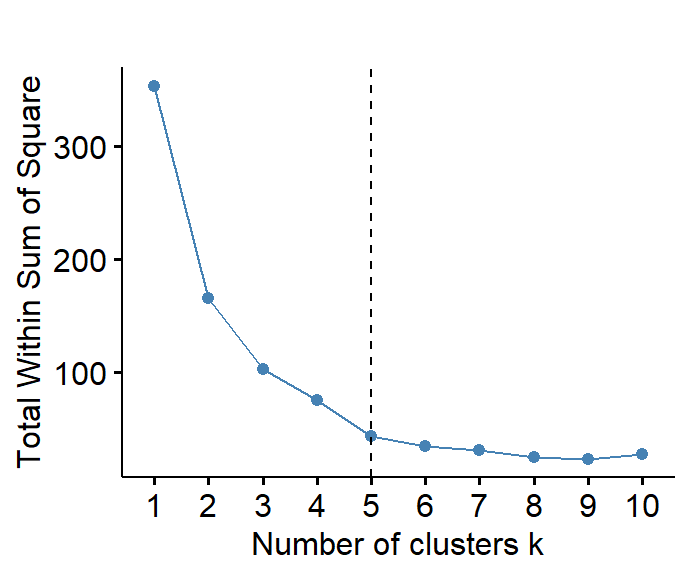
Figure 1: Estmation of the optimum number of clusters for CLR-transformed urban land-use data.
We have indicated, in Figure 1, five clusters for the cities data,
based on visual identification of a break in the slope of the WSS
vs. 'Number of clusters' curve (obviously this is somewhat
subjective). In the following analyses we will assume the same number of
clusters (K = 5) for K-means clustering.
Compute K-means clustering for open data
data0 <- na.omit(cities_clr[,c("sType","Compact","Open","Lightweight","Industry")])
data0[,c("Compact","Open","Lightweight","Industry")] <-
  scale(data0[,c("Compact","Open","Lightweight","Industry")])
set.seed(123)
cities_open_kmeans <- kmeans(data0[,2:NCOL(data0)], 5, nstart = 25)
cat("components of output object are:\n")
ls(cities_open_kmeans)
cat("\nK-means clustering with",length(cities_open_kmeans$size),
    "clusters of sizes",cities_open_kmeans$size,"\n\n")
cat("Cluster centers (scaled to z-scores) in K-dimensional space:\n")
cities_open_kmeans$centers
outtable <- data.frame(Cluster = seq(1,length(cities_open_kmeans$size),1),
                       Cities = rep("nil",length(cities_open_kmeans$size)))
## components of output object are:
## [1] "betweenss" "centers" "cluster" "ifault" "iter" "size"
## [7] "tot.withinss" "totss" "withinss"
##
## K-means clustering with 5 clusters of sizes 18 10 7 4 1
##
## Cluster centers (scaled to z-scores) in K-dimensional space:
## Compact Open Lightweight Industry
## 1 0.2104279 0.4402114 -0.3639952 -0.1623997
## 2 0.9635293 -1.0288909 -0.3534227 0.4534289
## 3 -0.7512239 0.7952617 -0.2848469 0.7996505
## 4 -1.0301901 -1.3458683 2.7726291 -2.2588450
## 5 -4.0436668 2.1817461 0.9895518 1.8267321
The output object from the kmeans function is a list
which contains the information we're interested in: the sum-of-squares
between and within clusters (betweenss,
tot.withinss, totss, withinss),
the location in K dimensions of the centers of the clusters
(centers), the assignment of each observation to a cluster
(cluster), the number of observations in each cluster
(size), and the number of iterations taken to find the
solution (iter).
Cluster | Cities |
|---|---|
Cluster 1 | New York Sao Paulo Beijing Paris Sydney Istanbul Milan Washington DC Qingdao Berlin Madrid Changsha Rome Lisbon Dongying Shenzhen Zurich Hong Kong |
Cluster 2 | Jakarta Guangzhou Melbourne Cairo Santiago de Chile Vancouver Tehran San Francisco Rio de Janeiro Kyoto |
Cluster 3 | Shanghai London Moscow Nanjing Wuhan Amsterdam Munich |
Cluster 4 | Cape Town Mumbai Islamabad Nairobi |
Cluster 5 | Cologne |
Applying K-means clustering with 5 clusters to the open cities land-use data results in one larger cluster of 18 cities (Cluster 1). There are three medium clusters containing 1-10 cities (2-4), and cluster 5 has a single city. From the table of cluster centers, we get might conclude that:
- 18 Cluster 1 cities have a more even mix of land uses
- 10 Cluster 2 cities have greater Compact, and lower Open, land uses
- 7 Cluster 3 cities have an even mix of land uses with less compact and more Open than Cluster 1
- 4 Cluster 4 cities have greater Lightweight, and somewhat lesser Open land use
- The 1 Cluster 5 city has greater Industry, and lower Compact, land use
An interesting question to ask is whether the clusters are similar to
the categories we already have in the dataset (Type,
Global, and Region). The following plot
includes labelling to help us see the relationship of K-means clusters
to the Type category.
To represent clustering in 3 or more dimensions in a plot, we can use
principal components to reduce the number of dimensions, but still
retain information from all the variables. This is done very nicely by
the fviz_cluster() function from the R package
factoextra (Kassambara and Mundt, 2020).
[The output
from fviz_cluster is a ggplot; we don't do it
here, but for more efficient presentation and comparison, we would save
the ggplot2 output to objects, and plot these together using the
ggarrange() function from the ggpubr R
package.]
Plot kmeans clusters showing factor categories
row.names(data0) <- paste0(data0$sType,seq(1,NROW(data0)))
fviz_cluster(cities_open_kmeans, data = data0[,2:NCOL(data0)],
             palette = c("#800000", "#E7B800", "#FC4E07","purple2","darkcyan"),
             labelsize=10, main = "",
             ellipse.type = "euclid", # Concentration ellipses
             star.plot = TRUE, # Add segments from centroids to items
             repel = T,        # if true avoids label overplotting (can be slow)
             ggtheme = theme_bw())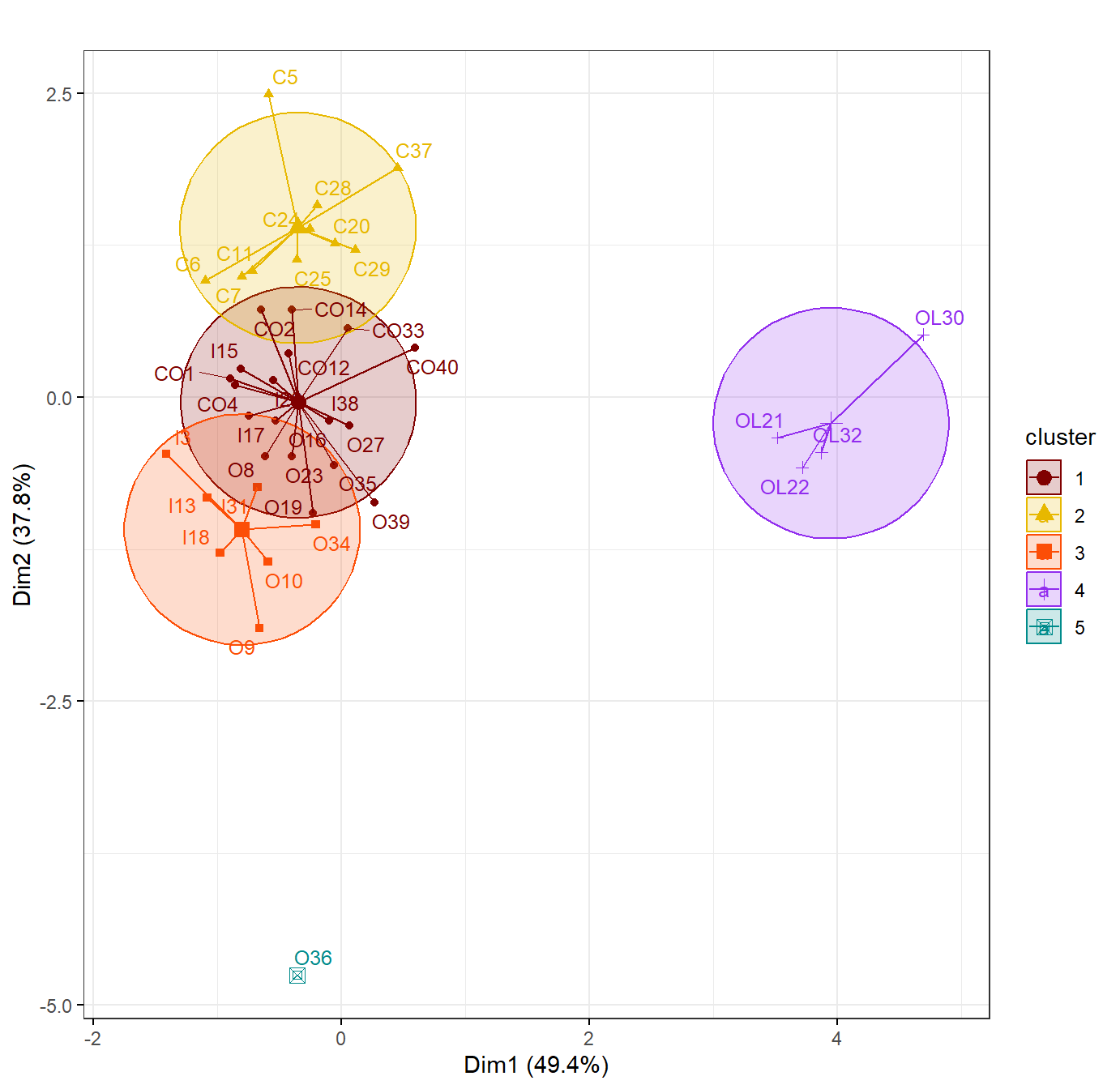
Figure 2: K-means cluster plotm for CLR-transformed (opened) urban land-use data.
From the plot in Figure 2 we can see that, for both the cities land
use data, K-means clustering did not produce clusters that overlap
convincingly with the city Type category in our data. There is some
differentiation; for example there is a cluster (cluster 4) composed
only of Open-Lightweight (OL) cities. We haven't checked the
relationship of the other categories (Global,
Region) to the clusters obtained, but some editing of the
code would answer this question for us!
Hierarchical Clustering
Hierarchical clustering is another unsupervised
classification method, which groups observations into successively
larger clusters (i.e. hierarchically) depending on their
multivariate similarity or dissimilarity. The procedure first
requires generation of a distance matrix (we use the
get_dist() function from the factoextra
package), following which the clustering procedure can begin.
Create dissimilarity (distance) matrix
dataHC <- na.omit(cities_clr[,c("City","sType","Compact","Open","Lightweight","Industry")])
row.names(dataHC) <- paste0(dataHC$City, " ", "(", dataHC$sType, seq(1,NROW(dataHC)), ")")
dataHC$City <- NULL
dataHC$sType <- NULL
cities_open_diss <- get_dist(scale(dataHC), method = "euclidean")
cat("First 8 rows and first 4 columns of distance matrix:\n")
round(as.matrix(cities_open_diss)[1:8, 1:4], 2)
## First 8 rows and first 4 columns of distance matrix:
## New York (CO1) Sao Paulo (CO2) Shanghai (I3) Beijing (CO4)
## New York (CO1) 0.00 0.64 1.44 0.08
## Sao Paulo (CO2) 0.64 0.00 1.95 0.67
## Shanghai (I3) 1.44 1.95 0.00 1.46
## Beijing (CO4) 0.08 0.67 1.46 0.00
## Jakarta (C5) 3.36 3.10 3.30 3.42
## Guangzhou (C6) 1.60 1.61 1.47 1.67
## Melbourne (C7) 1.10 0.91 1.65 1.16
## Paris (O8) 0.75 1.22 1.65 0.67The distance matrix, part of which (the 'top-left' corner) is shown
here, shows the distance in terms of the measurement variables between
any pair of points. In this case the variables are
Compact,Open,Lightweight,and
Industry, so the resulting 4-dimensional space is hard to
visualise, but for Euclidean distance used here it represents
the equivalent of straight-line distance between each observation, each
defined by a 4-dimensional vector. There are several other ways to
define distance (or (dis)similarity) which are used in various
disciplines, such as Manhattan, Jaccard, Bray-Curtis, Mahalonobis (and
others based on covariance/correlation), or Canberra. [Try running
?factoextra::dist and read the information for
method for additional information.]
Perform hierarchical clustering for closed data
The hierarchical clustering algorithm: (1) assigns
each observation to its own cluster, each containing only one
observation. So, at the beginning, the distances (or (dis)similarities)
between the clusters is the same as the distances between the items they
contain. (2) The closest pair of clusters is then
computed, and this pair is merged into a single cluster.
(3) Distances are re-calculated between the new cluster
and each of the old clusters, and steps 2 and 3 are repeated until all
items are clustered into a single cluster. Finally, now the algorithm
has generated a complete hierarchical tree, we can split the
observations into k clusters by separating them at the
k-1 longest branches (for our data, see Figure 3).
Since the clusters are a group of points rather than single points,
there are several ways of combining the observations into clusters – run
?stats::hclust and see under 'method' for more
information.
Assess the validity of the cluster tree
# For open data:
cities_open_coph <- cophenetic(cities_open_hc)
cat("Correlation coefficient r =",cor(cities_open_diss,cities_open_coph),"\n")
cat("\nRule-of-thumb:\n",
 "Cluster tree represents actual distance matrix accurately enough if r > 0.75\n")
## Correlation coefficient r = 0.8650444
##
## Rule-of-thumb:
## Cluster tree represents actual distance matrix accurately enough if r > 0.75
The cophenetic distance may be considered a 'back
calculation' of the distance matrix based on the dendrogram (run
?cophenetic for more details). We then calculate a
correlation coefficient between the actual distance matrix and the
cophenetic distance matrix. If the correlation is great enough
(nominally > 0.75), we assume that the dendrogram adequately
represents our data. (If the actual vs. cophenetic correlation
is too low, we may want to choose another distance measure, or a
different hierarchical clustering algorithm.) Our results show that the
dendrogram for our data is an adequate representation of the applicable
distance matrix.
plot(cities_open_hc, cex=0.8, main="")
abline(h = c(2.2,2.8,4.1), col = c("blue2","purple","red3"), lty = c(2,5,1))
text(c(38,38,38),c(2.2,2.8,4.1), pos=3,
     col=c("blue2","purple","red3"), offset = 0.2,
     labels=c("Cut for 5 clusters","Cut for 4 clusters","Cut for 3 clusters"))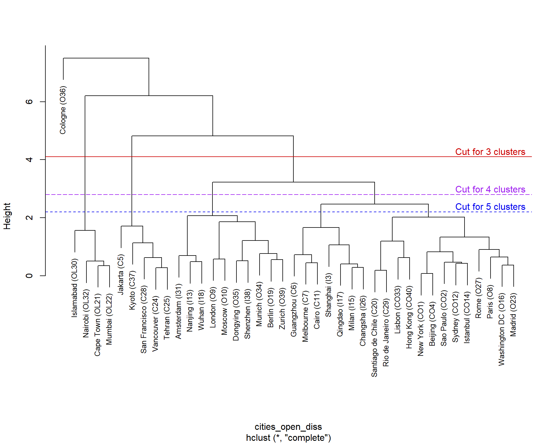
Figure 3: Hierarchical cluster dendrogram for open (CLR-transformed) urban land-use data.
The plot in Figure 3 is a hierarchical clustering 'tree', or dendrogram. We can see that the lowest order clusters, joined above the variable names, contain two observations (cities, in this dataset), reflecting the first iteration of Step 2 in the clustering algorithm described above. As we look higher in the dendrogram, we see additional observations or clusters grouped together, until at the highest level a single grouping exists. 'Cutting' the dendrogram at different heights will result in different numbers of clusters; the lower the cut level, the more clusters we will have. For the cities data we have shown cuts in Figure 3 resulting in 3, 4, or 5 clusters. There are numerous ways to decide where to make the cut; for some of these, see Kassambara (2018).
Find the optimum number of clusters
We did a similar analysis on the same dataset (cities land-use) for
K-means clustering, estimating the optimum number of clusters using the
'weighted sum-of-squares' (wss) method. In Figure 4 we
estimate the best cluster numbers using another common method, the
silhouette method.
#
require(factoextra)
data0 <- na.omit(cities_clr[,c("Compact","Open","Lightweight","Industry")])
fviz_nbclust(data0, hcut, method="silhouette", verbose=F) +
  labs(title="")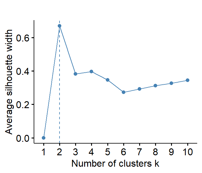
Figure 4: Estmation of the optimum number of clusters by the silhouette method for open (CLR-transformed) urban land-use data.
We can also assess optimum cluster numbers using the NbClust() function in the 'NbClust' package:
cat("Open CLR data:\n")
NbClust::NbClust(data=cities_clr[,c("Compact","Open","Lightweight","Industry")],
                 distance = "euclidean", min.nc = 2, max.nc = 15,
                 method = "complete", index = "silhouette")
## Open CLR data:
## $All.index
## 2 3 4 5 6 7 8 9 10 11 12 13 14 15
## 0.6030 0.7011 0.4118 0.3173 0.3097 0.3147 0.2946 0.3140 0.3474 0.3426 0.3722 0.4034 0.4243 0.4317
##
## $Best.nc
## Number_clusters Value_Index
## 3.0000 0.7011
##
## $Best.partition
## New York Sao Paulo Shanghai Beijing Jakarta
## 1 1 1 1 1
## Guangzhou Melbourne Paris London Moscow
## 1 1 1 1 1
## Cairo Sydney Nanjing Istanbul Milan
## 1 1 1 1 1
## Washington DC Qingdao Wuhan Berlin Santiago de Chile
## 1 1 1 1 1
## Cape Town Mumbai Madrid Vancouver Tehran
## 2 2 1 1 1
## Changsha Rome San Francisco Rio de Janeiro Islamabad
## 1 1 1 1 2
## Amsterdam Nairobi Lisbon Munich Dongying
## 1 2 1 1 1
## Cologne Kyoto Shenzhen Zurich Hong Kong
## 3 1 1 1 1
Note that there are very many
combinations of making a distance matrix and clustering
methods! See ?NbClust::NbClust for a list of
possibilities.
Cut dendrogram into clusters
This was illustrated in Figure 3 above, and we now investigate the clustering in more detail, assuming 4 clusters.
cities_open_grp <- cutree(cities_open_hc, k = 4)
tccg <- data.frame(table(cities_open_grp))
outtable <- data.frame(Cluster = seq(1,nlevels(as.factor(cities_open_grp))),
                       Cities = rep("nil",nlevels(as.factor(cities_open_grp))),
                       Freq = rep(0,nlevels(as.factor((cities_open_grp)))))
for (i in 1:nlevels(as.factor(cities_open_grp))) {
  outtable[i,1] <- paste("Cluster",i)
  outtable[i,2] <- paste(names(which(cities_open_grp==i)),
                         collapse = " ")
  outtable[i,3] <- as.numeric(tccg[i,2])}
flextable(outtable) |>
  theme_zebra(odd_header = "#D0E0FF") |>
  border_outer(border=BorderDk, part = "all") |>
  width(j=1:3, width=c(2.5,12.5,2.5), unit = "cm") |>
set_caption(caption="Table 2: Cities in each hierarchical cluster from analysis of open (CLR-transformed) data.")Cluster | Cities | Freq |
|---|---|---|
Cluster 1 | New York (CO1) Sao Paulo (CO2) Shanghai (I3) Beijing (CO4) Guangzhou (C6) Melbourne (C7) Paris (O8) London (O9) Moscow (O10) Cairo (C11) Sydney (CO12) Nanjing (I13) Istanbul (CO14) Milan (I15) Washington DC (O16) Qingdao (I17) Wuhan (I18) Berlin (O19) Santiago de Chile (C20) Madrid (O23) Changsha (I26) Rome (O27) Rio de Janeiro (C29) Amsterdam (I31) Lisbon (CO33) Munich (O34) Dongying (O35) Shenzhen (I38) Zurich (O39) Hong Kong (CO40) | 30 |
Cluster 2 | Jakarta (C5) Vancouver (C24) Tehran (C25) San Francisco (C28) Kyoto (C37) | 5 |
Cluster 3 | Cape Town (OL21) Mumbai (OL22) Islamabad (OL30) Nairobi (OL32) | 4 |
Cluster 4 | Cologne (O36) | 1 |
The decision to cut the dendrograms into 4 clusters (i.e. at a level which intersects exactly 4 'branches') is somewhat subjective, but could be based on other information such as K-means clustering, PCA, or pre-existing knowledge of the data.
A diagram comparing the clusters in cut dendrograms for closed and open data is shown below, in Figure 5.
Plot dendrograms with cuts
fviz_dend(cities_open_hc, k = 4, # Cut in five groups
          main = "", ylab="", cex = 0.7, # label size
          k_colors = c("gray40","red3", "blue2", "purple"),
          color_labels_by_k = TRUE, # color labels by groups
          rect = TRUE, # Add rectangle around groups
          labels_track_height = 10 # adjust low margin for long labels
)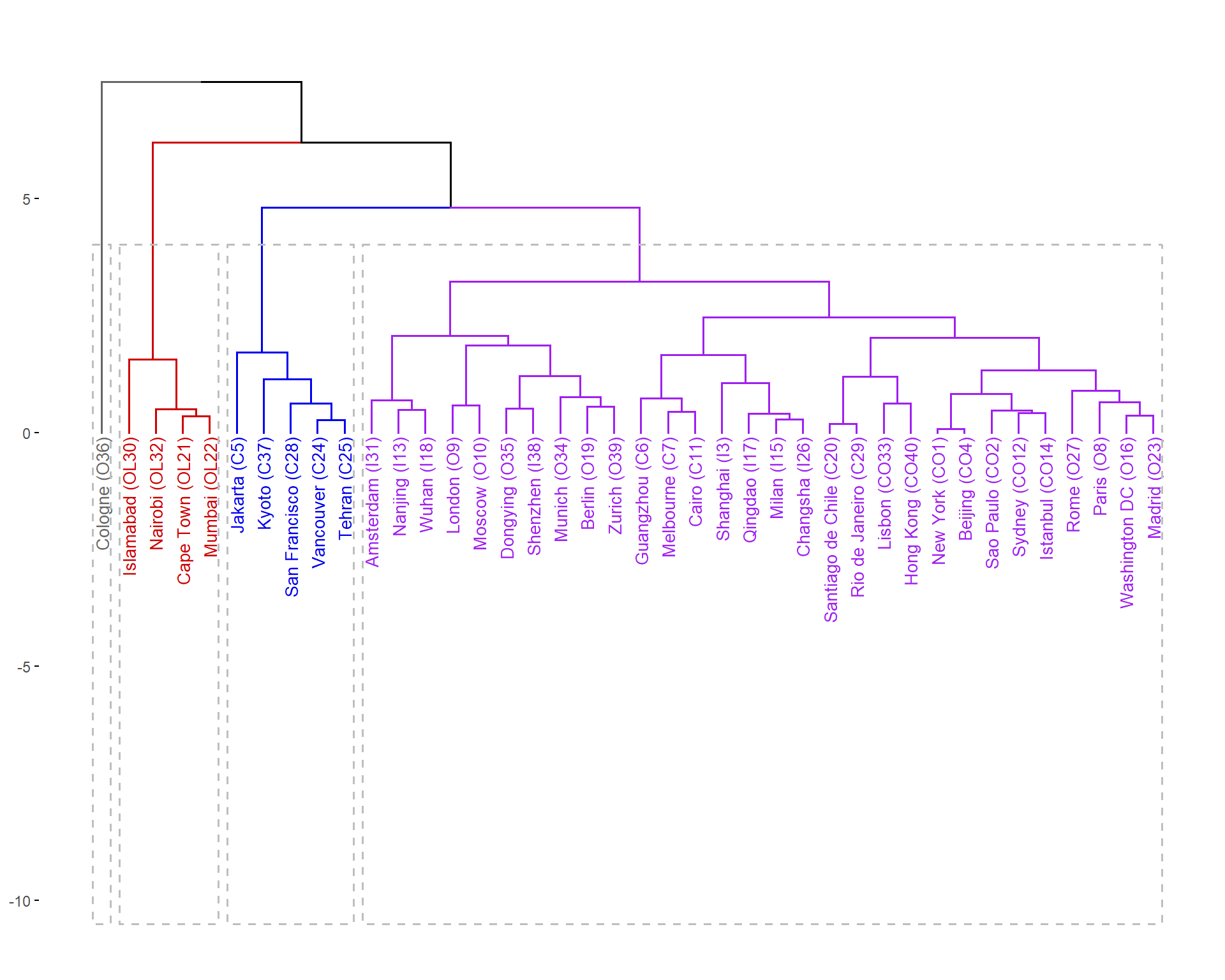
Figure 5: Hierarchical cluster dendrograms for CLR-transformed (open) urban land-use data, showing clusters within dashed rectangles.
This session has shown us how to apply two unsupervised classification methods, K-means clustering and hierarchical clustering, to a compositional dataset containing cities land-use data.
References and R Packages
Hu, J., Wang, Y., Taubenböck, H., Zhu, X.X. (2021). Land consumption in cities: A comparative study across the globe. Cities, 113: 103163, https://doi.org/10.1016/j.cities.2021.103163.
Kassambara, A. (2018). Determining The Optimal Number Of Clusters: 3 Must Know Methods. Datanovia, Montpellier, France. (https://www.datanovia.com/en/lessons/determining-the-optimal-number-of-clusters-3-must-know-methods/)
Kassambara, A. and Mundt, F. (2020). factoextra: Extract and Visualize the Results of Multivariate Data Analyses. R package version 1.0.7. https://CRAN.R-project.org/package=factoextra
Maechler, M., Rousseeuw, P., Struyf, A., Hubert, M., Hornik, K.(2021). cluster: Cluster Analysis Basics and Extensions. R package version 2.1.2. https://CRAN.R-project.org/package=cluster
Reimann, C., Filzmoser, P., Garrett, R. G., & Dutter, R. (2008). Statistical Data Analysis Explained: Applied Environmental Statistics with R (First ed.). John Wiley & Sons, Chichester, UK.
Venables, W. N. & Ripley, B. D. (2002) Modern Applied Statistics with S (MASS). Fourth Edition. Springer, New York. ISBN 0-387-95457-0. http://www.stats.ox.ac.uk/pub/MASS4/
Wickham, H. (2019). stringr: Simple, Consistent Wrappers for Common String Operations. R package version 1.4.0. https://CRAN.R-project.org/package=stringr
CC-BY-SA • All content by Ratey-AtUWA. My employer does not necessarily know about or endorse the content of this website.
Created with rmarkdown in RStudio. Currently using the free yeti theme from Bootswatch.