Statistics for Comparisons

Material to support teaching in Environmental Science at The University of Western Australia

Units ENVT3361, ENVT4461, and ENVT5503

Comparisons pages: Parametric tests | Non-parametric tests

Activities for this Workshop

Before you leave this week’s lab, make sure you know how and when to:

Use a non-parametric Wilcoxon test to compare the means of 2 groups of a variable
(i.e. categorised with a 2-level factor)

estimate effect size

Use a non-parametric Kruskal-Wallis test to compare the means of 3 or more groups of a variable
(i.e. categorised with a ≥3-level factor)

conduct relevant pairwise comparisons

Make relevant high-quality graphics to illustrate means comparisons (e.g. box plots with means)

For parametric means comparisons we asked you to learn:

Use a single-sided t- test to compare the mean of a variable with a fixed value (e.g. an environmental guideline)
Use a two -sided Welch's t-test to compare the means of 2 groups of a variable (i.e. categorised with a two-two-level factor)
Calculate a Cohen's d effect size for a 2-group mean comparison
Make a new factor using the cut() function in R
Repeat 1 & 2 above using analysis of variance (ANOVA) to compare means for 3 or more groups.
Generate a pairwise comparison of means from the analysis in step 5.

Files and other learning materials

Supporting Information

📰Decision tree for means comparisons methods
(on UWA LMS, login needed)

Code and Data files

🔣 R code file for Workshop: Advanced Means Comparisons – for Week 6, start at Non-parametric tests (line 409)

📊Smith's Lake / Veryard Reserve data (sv2017) in CSV format

As usual, we first need to read the data and load the necessary packages:

sv2017 <- read.csv("sv2017_original.csv", stringsAsFactors = TRUE)
sv2017$Reserve <- cut(sv2017$Northing,
                      breaks = c(0,6466530,9999999),
                      labels = c("Smiths","Veryard"))
sv17_soil <- subset(sv2017, subset=sv2017$Type=="Soil")

library(car)
library(effsize)
library(rcompanion)
library(multcompView)
library(RcmdrMisc)

Non-Parametric Comparisons

We need to use a different type of statistical test if our variable(s) do not have a normal distribution (even when log₁₀- or power-transformed). The non-parametric tests are not based on the actual values of our variable, but are calculated using the ranking (numerical ordering) of each observation.

Note on parametric vs. non-parametric tests

There are arguments that the parametric tests (e.g. the t-test and analysis of variance we covered in an earlier session on means comparisons) can be used even if the distributions of variables are not normal. Some authors, however, recommend the use of parametric tests in most cases, based on

The tendency for the means subsamples of populations from non-normal distributions to be nornally distributed, regardless of the shape of the underlying distribution. This is the Central Limit Theorem - see this discussion by James Fogarty of UWA. Prof Fogarty et al. (2021) also mention that parametric tests have greater ability to detect differences if their assumptions are met.
The robustness of parametric methods in practice – see this page by John McDonald from the University of Delaware. Prof. McDonald states that “...one-way anova is not very sensitive to deviations from normality.”

We will continue to cover non-parametric comparison tests, but you can make up your own mind after doing your own research on the pros and cons.

1. Wilcoxon test

From previous sessions we know that most untransformed variables are not normally distributed. For comparison between exactly 2 groups we use the Wilcoxon rank-sum test (via the wilcox.test() function). The Wilcoxon test is based on ranking of observations, so should be independent of transformation – as in the example below:

wilcox.test(sv17_soil$Na ~ sv17_soil$Reserve)
{cat("Means for original (untransformed) variable\n")
meansNa <- tapply(sv17_soil$Na, sv17_soil$Reserve, mean,
                  na.rm=TRUE)
print(signif(meansNa, 3))
cat("\n--------------------------------------------\n")}
wilcox.test(sv17_soil$Na.pow ~ sv17_soil$Reserve)
{cat("Means for transformed variable\n")
meansNa <- tapply(sv17_soil$Na.pow, sv17_soil$Reserve, mean, na.rm=TRUE)
print(signif(meansNa, 3))}
rm(meansNa) # remove temporary object(s)


    Wilcoxon rank sum test with continuity correction

data:  sv17_soil$Na by sv17_soil$Reserve
W = 246, p-value = 0.01426
alternative hypothesis: true location shift is not equal to 0

Means for original (untransformed) variable
 Smiths Veryard 
    102     139 

--------------------------------------------

    Wilcoxon rank sum test with continuity correction

data:  sv17_soil$Na.pow by sv17_soil$Reserve
W = 246, p-value = 0.01426
alternative hypothesis: true location shift is not equal to 0

Means for transformed variable
 Smiths Veryard 
   1.76    1.85

The output of wilcox.test() above shows a p-value < 0.05, so we reject H₀ (that the rank sum of each group is not different from a case where the ranks of each group are randomly ordered). In rejecting H₀ we can accept the alternative hypothesis, that the distribution of one group is shifted relative to the other.

It's somewhat important to recognise that the Wilcoxon rank-sum test does not compare means (or even medians). Based on the rank sums of the variable tested, the Wilcoxon rank-sum test simply tests whether or not the distribution in one group is shifted relative to the other group. If the distributions in each group have identical shapes, than we can say that the Wilcoxon test compares medians, but since the distributions are not often identical, our only conclusions should be about the 'location shift' of one group's distribution relative to the other.

The quantity compared in the Wilcoxon test is the mean rank sum – the sum of the ranks for all observations in a group, divided by the number of observations in that group.

data0 <- na.omit(sv17_soil[,c("Reserve","Na")])
data0 <- data0[order(data0$Na),] ; row.names(data0) <- NULL
par(mar=c(3,3,.5,.5), mgp=c(1.5,0.2,0),tcl=0.2,font.lab=2,las=0)
with(data0, boxplot(Na ~ Reserve))
with(data0, stripchart(Na ~ Reserve, vertical=TRUE, add=TRUE, method="jitter",
                        pch = 19, cex=0.5, col=c("#00308780","#faaa0080")))

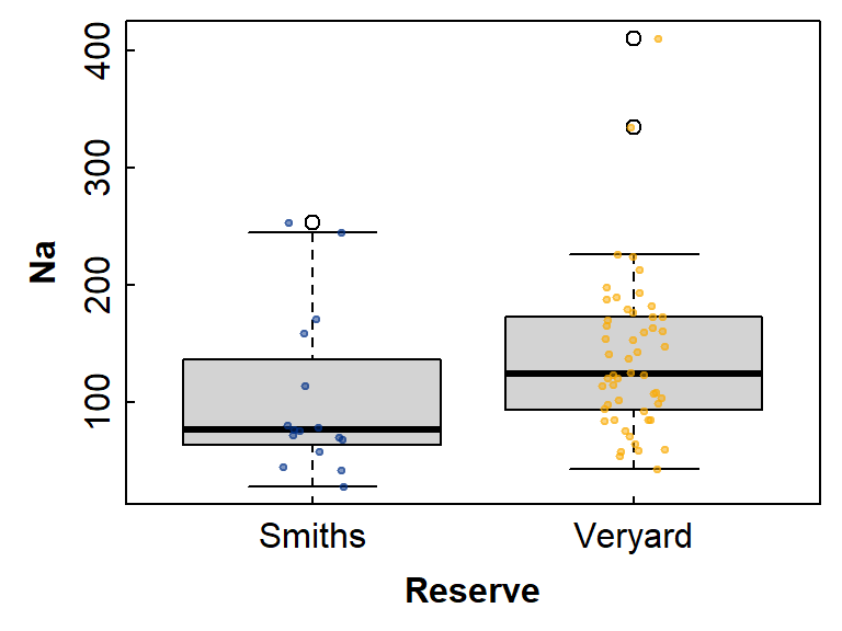
Figure 1: Boxplot showing differences in Na between groups defined by Reserve, with overplotted individual observations.

Figure 2: Na concentration ranks, the basis for the Wilcoxon rank-sum test, in soil in each reserve area, sampled at Smith's Lake and Charles Veryard Reserves in 2017.

Effect size

The test we need to use for effect size to accompany rank-based tests like wilcox.test() is not Cohen's d as we use to follow parametric tests. Non-parametric effect size tests are available in the effectsize R package – we need the rank_biserial() test (also called cliffs_delta()) for a 2-level comparison.

require(effectsize)
(rbsNa <- rank_biserial(sv17_soil$Na ~ sv17_soil$Reserve, verbose=F)); cat("\n")
interpret_rank_biserial(rbsNa$r_rank_biserial)

r (rank biserial) |         95% CI
----------------------------------
-0.41             | [-0.64, -0.11]

[1] "very large"
(Rules: funder2019)

2. Kruskal-Wallis test

We use the Kruskal-Wallis test (via the kruskal.test() function) for non-parametric comparisons between three or more groups defined by a factor.

This example is testing differences in Fe between sample Types in the complete Smith's – Veryard 2017 dataset.

kruskal.test(sv2017$Fe ~ sv2017$Type)
meansFe <- tapply(sv2017$Fe, sv2017$Type, mean,
                  na.rm=TRUE)
cat("Means for untransformed variable\n")
print(signif(meansFe),4)
rm(meansFe)


    Kruskal-Wallis rank sum test

data:  sv2017$Fe by sv2017$Type
Kruskal-Wallis chi-squared = 8.222, df = 2, p-value = 0.01639

Means for untransformed variable
   Sediment        Soil Street dust 
       5111        2695        3694

The output from kruskal.test() shows that H₀ can be rejected, so we can say the mean rank sums of each group defined by Type are significantly different.

We should note that the Kruskal-Wallis test does not compare means, and would only compare medians if the distributions in each group were the same shape. The Kruskal-Wallis test is based on the actual and expected values of the mean rank sum in each group, i.e., the sum of the ranks in a group divided by the number of observations in that group (as for the Wilcoxon test).

par(mar=c(3,3,.5,.5), mgp=c(1.5,0.2,0),tcl=0.2,font.lab=2,las=0)
with(sv2017, boxplot(Fe ~ Type, log="y", xlab="Sample Type", ylab = "Fe (mg/kg)"))
with(sv2017, stripchart(Fe ~ Type, vertical=TRUE, add=TRUE, method="jitter",
                        pch = 19, cex=0.5, col=c("#00308780","#faaa0080","#60008080")))

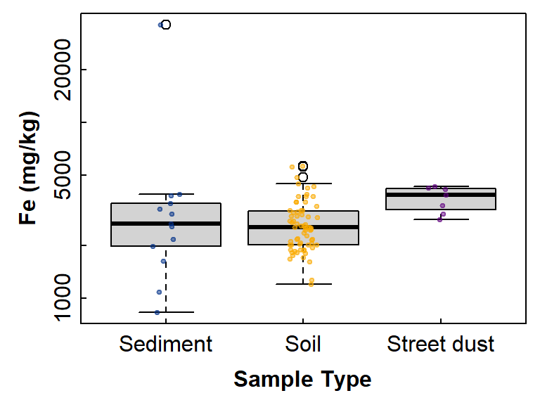
Figure 3: Boxplot showing differences in Fe between groups defined by Type, with overplotted individual observations.

With a p-value of ≈ 0.016, H₀ can be rejected. We still have the problem of not knowing which means are significantly different from each other. There are several options for pairwise comparisons of means following statistically significant Kruskal-Wallis results; we will use the pairwise Wilcoxon test (pairwise.wilcox.test()), for consistency with the 2-level comparisons in the previous section. Also, we should still be using a non-parametric test to match the original Kruskal-Wallis test. (More rigorous tests, such as Dunn's non-parametric all-pairs comparison test, are available in the R package PMCMRplus).

Figure 4: Fe concentration ranks (the basis for the Kruskal-Wallis test) in sediment, soil, and street dust sampled at Smith's Lake and Charles Veryard Reserves in 2017.

Pairwise comparisons following a Kruskal-Wallis test


    Pairwise comparisons using Wilcoxon rank sum test with continuity correction 

data:  Fe and Type 

            Sediment Soil 
Soil        0.743    -    
Street dust 0.091    0.012

P value adjustment method: holm

The pairwise comparisons show that only Soil and Street dust have significantly different Fe concentration. Note the p-value adjustment – we still use Holm's for multiple non-parametric comparisons.

We can also get a pairwise compact letter display based on the results of non-parametric tests. As before, we need the R packages rcompanion and multcompView to do this easily.

require(rcompanion)
require(multcompView)
pwFe_Type <- with(sv2017, pairwise.wilcox.test(Fe, Type)) 
pwFe_Type_pv <- fullPTable(pwFe_Type$p.value)               # from rcompanion
multcompLetters(pwFe_Type_pv)                               # from multcompView

   Sediment        Soil Street dust 
       "ab"         "a"         "b"

The output from pairwise.wilcox.test() shows that p ≤ 0.05 only for the Soil-Street dust comparison ("ab" matches "a" OR "b"). We can't reject H₀ for any other pairwise comparisons.

Effect sizes for the Kruskal-Wallis test

The effect size test to accompany a Kruskal-Wallis test is the rank_epsilon_squared() test in the effectsize R package

(resFe <- rank_epsilon_squared(sv2017$Fe, sv2017$Type, verbose = FALSE))
cat("\n\n") # blank output line
interpret_epsilon_squared(resFe$r)

Epsilon2 (rank) |       95% CI
------------------------------
0.09            | [0.05, 1.00]

- One-sided CIs: upper bound fixed at [1.00].

[1] "medium"
(Rules: field2013)

References and R Packages

Cohen, J. (1988). Statistical power analysis for the behavioral sciences (2^nd ed.). New York:Academic Press.

Fogarty, J.J., Rensing, K., & Stuckey, A. (2021). Introduction to R and Statistics: UWA School of Agriculture and Environment. https://saestatsteaching.tech/

McDonald, J.H. (2014). Kruskal–Wallis test. In Handbook of Biological Statistics (3^rd ed.). Sparky House Publishing, Baltimore, Maryland. https://www.biostathandbook.com/kruskalwallis.html

Sawilowsky, S.S. (2009). New Effect Size Rules of Thumb. Journal of Modern Applied Statistical Methods 8:597-599.

Run the R code below to get citation information for the R packages used in this document.

citation("car", auto = TRUE)
citation("RcmdrMisc", auto = TRUE)
citation("effectsize", auto = TRUE)
citation("multcomp", auto = TRUE)
citation("PMCMRplus", auto = TRUE)
citation("rcompanion", auto = TRUE)
citation("multcompView", auto = TRUE)

To cite package 'car' in publications use:

  Fox J, Weisberg S, Price B (2023). _car: Companion to Applied Regression_. R package
  version 3.1-2, <https://CRAN.R-project.org/package=car>.

A BibTeX entry for LaTeX users is

  @Manual{,
    title = {car: Companion to Applied Regression},
    author = {John Fox and Sanford Weisberg and Brad Price},
    year = {2023},
    note = {R package version 3.1-2},
    url = {https://CRAN.R-project.org/package=car},
  }
To cite package 'RcmdrMisc' in publications use:

  Fox J, Marquez M (2023). _RcmdrMisc: R Commander Miscellaneous Functions_. R package
  version 2.9-1, <https://CRAN.R-project.org/package=RcmdrMisc>.

A BibTeX entry for LaTeX users is

  @Manual{,
    title = {RcmdrMisc: R Commander Miscellaneous Functions},
    author = {John Fox and Manuel Marquez},
    year = {2023},
    note = {R package version 2.9-1},
    url = {https://CRAN.R-project.org/package=RcmdrMisc},
  }
To cite package 'effectsize' in publications use:

  Ben-Shachar M, Makowski D, Lüdecke D, Patil I, Wiernik B, Thériault R, Waggoner P
  (2024). _effectsize: Indices of Effect Size_. R package version 0.8.9,
  <https://CRAN.R-project.org/package=effectsize>.

A BibTeX entry for LaTeX users is

  @Manual{,
    title = {effectsize: Indices of Effect Size},
    author = {Mattan S. Ben-Shachar and Dominique Makowski and Daniel Lüdecke and Indrajeet Patil and Brenton M. Wiernik and Rémi Thériault and Philip Waggoner},
    year = {2024},
    note = {R package version 0.8.9},
    url = {https://CRAN.R-project.org/package=effectsize},
  }
To cite package 'multcomp' in publications use:

  Hothorn T, Bretz F, Westfall P (2023). _multcomp: Simultaneous Inference in General
  Parametric Models_. R package version 1.4-25,
  <https://CRAN.R-project.org/package=multcomp>.

A BibTeX entry for LaTeX users is

  @Manual{,
    title = {multcomp: Simultaneous Inference in General Parametric Models},
    author = {Torsten Hothorn and Frank Bretz and Peter Westfall},
    year = {2023},
    note = {R package version 1.4-25},
    url = {https://CRAN.R-project.org/package=multcomp},
  }
To cite package 'PMCMRplus' in publications use:

  Pohlert T (2023). _PMCMRplus: Calculate Pairwise Multiple Comparisons of Mean Rank
  Sums Extended_. R package version 1.9.10,
  <https://CRAN.R-project.org/package=PMCMRplus>.

A BibTeX entry for LaTeX users is

  @Manual{,
    title = {PMCMRplus: Calculate Pairwise Multiple Comparisons of Mean Rank Sums
Extended},
    author = {Thorsten Pohlert},
    year = {2023},
    note = {R package version 1.9.10},
    url = {https://CRAN.R-project.org/package=PMCMRplus},
  }
To cite package 'rcompanion' in publications use:

  Mangiafico S (2024). _rcompanion: Functions to Support Extension Education Program
  Evaluation_. R package version 2.4.36,
  <https://CRAN.R-project.org/package=rcompanion>.

A BibTeX entry for LaTeX users is

  @Manual{,
    title = {rcompanion: Functions to Support Extension Education Program Evaluation},
    author = {Salvatore Mangiafico},
    year = {2024},
    note = {R package version 2.4.36},
    url = {https://CRAN.R-project.org/package=rcompanion},
  }
To cite package 'multcompView' in publications use:

  Graves S, Piepho H, Dorai-Raj LSwhfS (2024). _multcompView: Visualizations of Paired
  Comparisons_. R package version 0.1-10,
  <https://CRAN.R-project.org/package=multcompView>.

A BibTeX entry for LaTeX users is

  @Manual{,
    title = {multcompView: Visualizations of Paired Comparisons},
    author = {Spencer Graves and Hans-Peter Piepho and Luciano Selzer with help from Sundar Dorai-Raj},
    year = {2024},
    note = {R package version 0.1-10},
    url = {https://CRAN.R-project.org/package=multcompView},
  }

ATTENTION: This citation information has been auto-generated from the package
DESCRIPTION file and may need manual editing, see 'help("citation")'.

CC-BY-SA • All content by Ratey-AtUWA. My employer does not necessarily know about or endorse the content of this website.
Created with rmarkdown in RStudio. Currently using the free yeti theme from Bootswatch.