What is R?

R is called a "statistical computing environment". This means two things:

R is software that allows us to perform statistical analysis of data;
R is a type of computer programming code (a language).

In R these two features are combined so that we perform the tasks we need to by writing instructions in R code. We commonly want to:

create or input data
format, store, and save our data
perform statistical and numerical analysis of our data
display our data and report our analysis in graphs and tables

By using R code to do this, we can easily reproduce our analyses, that is, use exactly the same procedures again on additional data, or simply re-create what we have done. We can save our R code in simple 'text' files, or even in a document called an R Notebook which uses a few additional coding features (called 'R markdown') to let us save our code and the results of our analysis in the same document. We use R markdown to produce documents such as reports (this document is created using R markdown).

"...R has developed into a powerful and much used open source tool ... for advanced statistical data analysis..."

— Reimann et al. (2008) – Statistical Data Analysis Explained: Applied Environmental Statistics with R, p.3.

R and RStudio

To make our job of using R easier, we'll be using the RStudio program. RStudio is an IDE or 'integrated development environment' which puts everything we need for R coding in one place, and has some helpful tools (such as predictive text for code, and some menu-driven functions) to make coding easier. In this document, when we say 'R', we really mean 'R in the RStudio environment'.

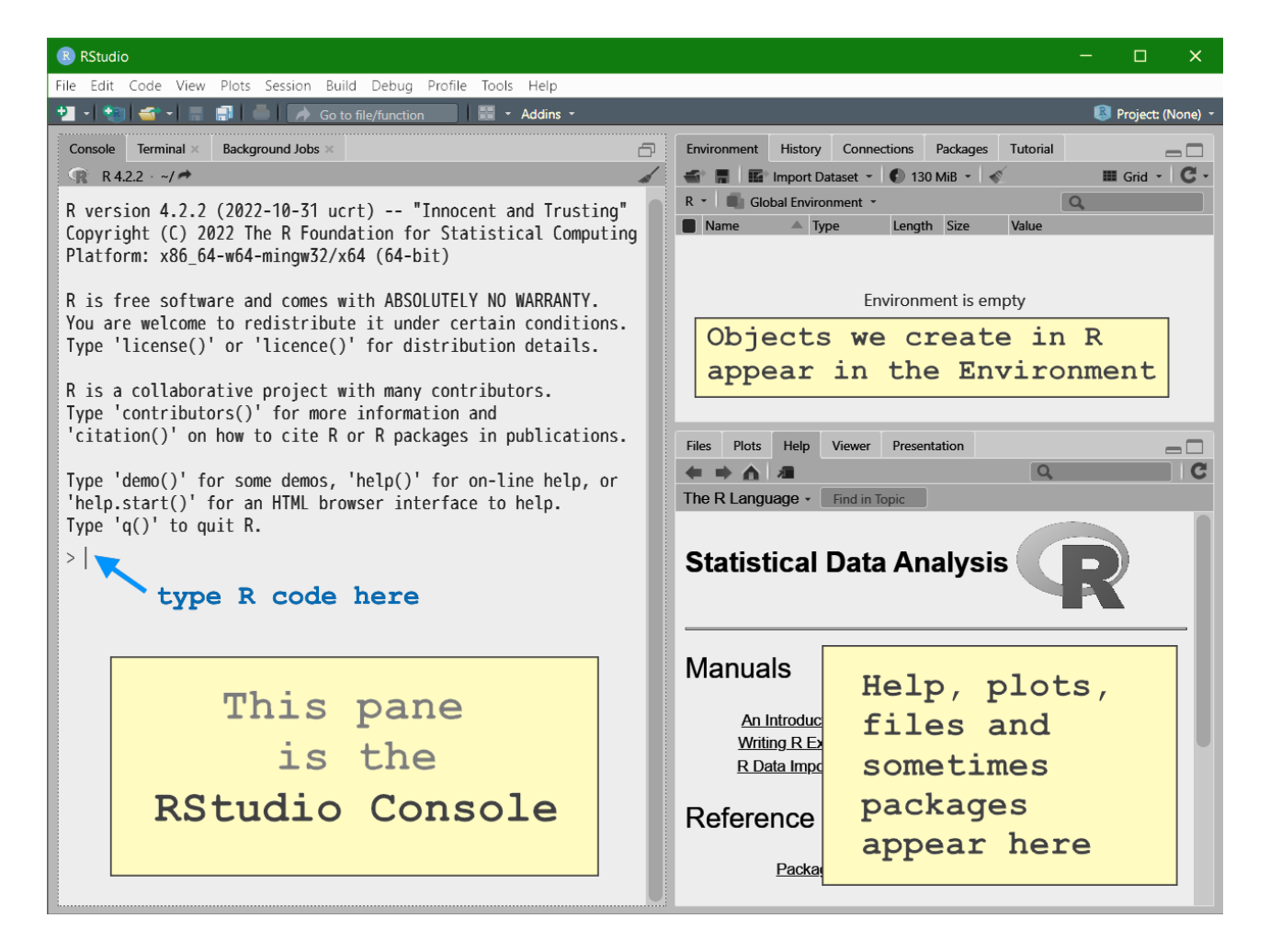
Figure 1: The RStudio window with a very brief explanation of some different sub-panes.

Three things we really need to know about using R

How data are stored. R can handle many different types of data, such as numbers, text, categories, spatial coordinates, images, and so on. R uses various types of objects to store different types of data in different ways.
Code-based instructions. If we want R to do something for us, we need to give it instructions. We do this in other software too, commonly by using a mouse or other pointing device to click and select options from a menu. For example, in R we can sort a table of data by writing the instructions in R code:

data_sorted <- data[order(data$column1, data$column2),]

You don't have to remember this (yet). The code here is also to illustrate that, in this document, R code will be shown in blocks like the one above having a shaded background and fixed-space font.

In Excel, we can do the same thing, but we would use a sequence of point-and-click operations, such as that shown below:

using the mouse to select the cells we want to sort;
clicking on the Data menu;
clicking on the Sort button;
choosing the column we want to sort by in the dialog box that appears;
clicking 'OK'.

(We did say three things.) R is very literal, and needs precise instructions to do everything. A small error in our code will mean we get wrong, or no, results. For example, all R code is case-sensitive. Also, if we don't tell R where to look for things, it won't try anywhere else just in case we might have intended another location!
Go here for a great page on common errors in R and how to fix them

Types of data we commonly use in R

Single numbers

R can work with single numbers, much like a complex calculator.

To "run" R code, we can type it into the RStudio Console and press the enter key. We will see the results of running the code also in the Console, below the code we just entered.

123 + 456

## [1] 579

sq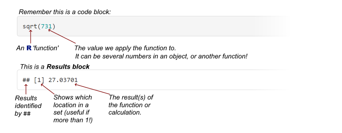rt(731)

## [1] 27.03701

Figure 2: Understanding simple R functions and output.

We don't usually use R like this, but it's handy to know that we have a calculator handy if we need in in the R Console!

R functions

This is also the place to introduce Functions in R. We just used a function – to calculate a square root: sqrt(731).

An R function is identified by a name such as sqrt, t.test or plot, followed by arguments in parentheses ( ) (the parentheses can be empty, for example help.start() – try it!). We used the argument 731 in the sqrt() function – some functions require several arguments, as you will see. Some arguments have default 'built-in' values.

There are huge numbers of built-in functions in R which we can use after first installing R, "straight out of the box" (we call this "base R"). For instance, see the R reference card v2 by Matt Baggott.

If we can't find the functions we need, they may be available in R packages which are additional libraries of functions that we can install from within the R environment. A commonly used package is car, the companion to applied regression. We would install this into R using a function install.packages("car"), which stores the library on our device. To use the functions in the car package we would load the library into our R session by running library(car).

We can also write our own functions in R and we may show you examples of these as you progress through this course.

Vectors

A vector is a one-dimensional set of numbers, similar to a column or row of values in a spreadsheet. We use the simple function c() to combine, or put together, a set of values. The code below shows how we can make a vector object using the assign code <- to give our vector a name of our choice. Just by entering the vector object's name, we can then see its contents:

a <- c(1,3,5,7,9,2,4,6,8,10)
a

##  [1]  1  3  5  7  9  2  4  6  8 10

We can also check the type of object using the class() function, or using another function that asks if the object is in a specific class (e.g. is.vector() or is.character()).

class(a)

## [1] "numeric"

is.vector(a)

## [1] TRUE

is.character(a)

## [1] FALSE

We can also make use of the square brackets: remember from Figure 2 that the values in square brackets [ ] are the index for a set of values. For a vector, which is one dimensional, we just need one value in [ ] at the end of our object name to select particular values:

a[3]

## [1] 5

# we can also use a range of values
a[7:10]

## [1]  4  6  8 10

There are some other useful ways to make vectors in R, such as the functions seq() (sequence) and rep() (repeat) (and many others!). Try changing some of the code below and running it, to make sure you understand the results each time.

# make a vector with a sequence of numbers from 2 to 80 in steps of 2
b <- seq(2,80,2)
b

##  [1]  2  4  6  8 10 12 14 16 18 20 22 24 26 28 30 32 34 36 38 40 42 44 46 48 50 52 54 56 58 60
## [31] 62 64 66 68 70 72 74 76 78 80

Notice that if we have a long vector, the number in square brackets at the beginning of each line tells us which item the line starts with (i.e. its index).

# make a vector of the number 12 repeated 20 times
d <- rep(12,20)
d

##  [1] 12 12 12 12 12 12 12 12 12 12 12 12 12 12 12 12 12 12 12 12

Matrices

A matrix is a two-dimensional set of data with rows and columns. All of the entries must be the same type (e.g. integer, numeric, character). We can make a matrix using a vector (e.g. b from above), so long as we specify how many rows and/or columns we want:

m <- matrix(b, nrow = 5)
m

##      [,1] [,2] [,3] [,4] [,5] [,6] [,7] [,8]
## [1,]    2   12   22   32   42   52   62   72
## [2,]    4   14   24   34   44   54   64   74
## [3,]    6   16   26   36   46   56   66   76
## [4,]    8   18   28   38   48   58   68   78
## [5,]   10   20   30   40   50   60   70   80

By default we fill each column in order, but we can change this by using the byrow = TRUE option.

m <- matrix(b, ncol = 8, byrow = TRUE)
m

##      [,1] [,2] [,3] [,4] [,5] [,6] [,7] [,8]
## [1,]    2    4    6    8   10   12   14   16
## [2,]   18   20   22   24   26   28   30   32
## [3,]   34   36   38   40   42   44   46   48
## [4,]   50   52   54   56   58   60   62   64
## [5,]   66   68   70   72   74   76   78   80

We can locate each value in the matrix using a two-part index in square brackets [row, column]. Here are some examples (note that we always need the comma):

# single value at [row,column]
selection <- m[2,3] 
selection

## [1] 22

# a whole row by itself
selection <- m[4,]
selection

## [1] 50 52 54 56 58 60 62 64

# a whole column by itself
selection <- m[,8]
selection

## [1] 16 32 48 64 80

Data frames

Data frames are one of the most common ways to store data in R. They are two-dimensional like matrices, with rows and columns, but the columns can contain different types of data such as numbers (integer or numeric), text (character), or categories (factor), etc.

Data frame are one of the best ways to store "real" data which can contain information such as sample IDs, treatments, replicates, coordinates, categories, measurements, dates/times, etc. Let's make one and look at its properties.

df <- data.frame(Name = c("Sample 1","Sample 2","Sample 3","Sample 4","Sample 5"),
                 Group = as.factor(c("New","New","Old","Old","Old")),
                 Value = c(2.34,4.56,3.45,5.67,6.54),
                 Count = as.integer(c(21,35,19,18,27)))
df

##       Name Group Value Count
## 1 Sample 1   New  2.34    21
## 2 Sample 2   New  4.56    35
## 3 Sample 3   Old  3.45    19
## 4 Sample 4   Old  5.67    18
## 5 Sample 5   Old  6.54    27

We can see that we made a data frame 'df' with 4 columns and 5 rows (the first column of output is the row number, not part of the data frame's column count). All the columns contain a different type of information which we can see using the str() (structure) function:

str(df)

## 'data.frame':    5 obs. of  4 variables:
##  $ Name : chr  "Sample 1" "Sample 2" "Sample 3" "Sample 4" ...
##  $ Group: Factor w/ 2 levels "New","Old": 1 1 2 2 2
##  $ Value: num  2.34 4.56 3.45 5.67 6.54
##  $ Count: int  21 35 19 18 27

The output of str() shows that the column called Name contains chr (character = text) information, Group is a Factor (i.e. categorical information) with two levels or categories, Value is num (numeric = real numbers), and Count is int (integer).

Data frames are a very common way of storing our data in the R environment. The rows of our data frame represent our observations or 'samples'. The columns of a data frame are the variables – information about the samples which may be identifying information (character or categorical information), or measurements (usually numeric information such as counts or concentrations).

We should notice that each column name is preceded by a dollar sign $, and we also use this to specify single columns from a data frame:

# both lines of code below should give the same output!
df$Value

## [1] 2.34 4.56 3.45 5.67 6.54

df[,3]

## [1] 2.34 4.56 3.45 5.67 6.54

Other types of object in R

There are many other object types in R! Many of these are specialised to handle specific types of data, such as time series, spatial data, or raster images. One of the more common R objects is the list, which is a collection of different object types – often if we save the output of a function, it will be as an object of class list.

Working with files

Telling RStudio where to find our files

We've just seen how we can create data in R by typing it in, and some of our examples in class will do this, but the most common way of getting our data into R is to read (input) from a file.

Before we read any files, though, we need to tell R where to find the files we've saved, downloaded, or created. There are 2 ways to do this in RStudio:

In the top level menu, click Session » Set Working Directory » Choose Directory. This will open a window showing just folders (= directories). Click on the folder where your files are, and click the Open button.
With the RStudio Files pane already showing the files you are working with, click More ,
then Set As Working Directory .

Opening (and saving) a code file

If we write some code that works, it's good to save it so we can use it again or adapt it for a similar task. In classes, we will provide you with code files (having the extension .R) to help you learn what R code does.

To open a code file we have a few options:

just type ctrl-O, and choose the file from the 'Open file' window that appears
click on the open file icon, and choose the file from the 'Open file' window that appears
click on the file shown in the Files pane (lower right, see Figures 1 and 3) in the RStudio screen.

You can type code into a new file made by the keystroke combination ctrl-shift-N (for other new file types, use the RStudio menu File/New file).

Files can be saved by typing ctrl-S (you will be prompted for a new file name the first time you save a new file), or clicking the file-save icon.

Opening a data file

In classes, we will mainly supply data as CSV (Comma Separated Value, or .csv) files. These are a simple and widely-used way to store tabular data such as found in an R data frame, and can also be opened in Excel and other software.

R has a specific function for reading .csv files, read.csv(). If we know that our file contains categorical information present as text, we should also include the option stringsAsFactors = TRUE] (we can shorten TRUE to T).

df <- read.csv(file = "df.csv", stringsAsFactors = T)
df

##       Name Group Value Count
## 1 Sample 1   New  2.34    21
## 2 Sample 2   New  4.56    35
## 3 Sample 3   Old  3.45    19
## 4 Sample 4   Old  5.67    18
## 5 Sample 5   Old  6.54    27

If the file is not in our Working Directory, we would need to specify the whole path. We can also read directly from an internet address:

df <- read.csv(file = "C:/Users/neo/LocalData/R Projects/Learning R/df.csv",
               stringsAsFactors = T)
df <- read.csv("https://raw.githubusercontent.com/Ratey-AtUWA/learningR/main/df.csv",
               stringsAsFactors = T)

You might notice that we didn't include file = in the second example above. We can do this because file = is the option R expects first in the read.csv() function.

In general we can omit the option names in a function if we include the option values in the order that the function expects. It will help you remember what the code does, though, if you include the option names.

Saving and running code in files

In R we usually run code from a file rather than typing lines of code into the R Console. R code files that we provide for you to use will usually have the extension .R. We can:

Open files by clicking File/Open File... (or typing ctrl-O on the keyboard), then choosing from our computer or network file system
Create new .R code files by clicking File/New File/R Script (or typing ctrl-shift-N on the keyboard), then typing in code. Don't forget to save the file!

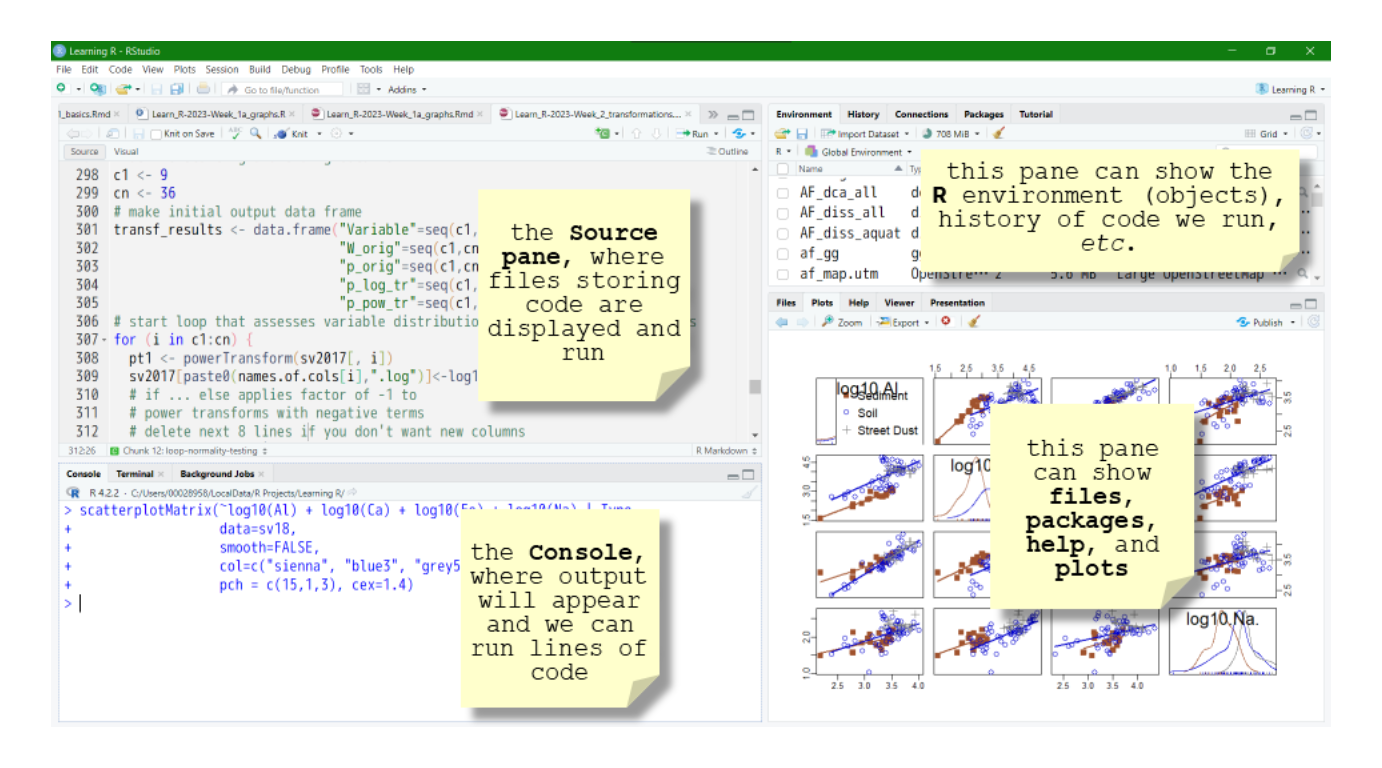
Figure 3: The RStudio window showing the Source sub-pane (and the other panes).

In an open R code file, we can run lines or chunks of code by selecting the code to be run with our pointing device, then clicking the ▮➨Run button at the top of the source pane, or typing ctrl-enter.
We can actually just put our cursor anywhere in a line of code and click ▮➨Run or type ctrl-enter.

Built-in R Help

How do we find out the order of options in a function? Well, R and RStudio have excellent Help utilities. For example, if we run the code help("read.csv") or just ?read.csv in the RStudio Console (usually the bottom-left pane), this will open the relevant help page in the Help pane at (lower) right. We can also search directly in the help pane.

If we're unsure about anything in R, especially, we may be able to find it in the Help system. A very useful place to start is by running the code below to get to the general help page:

help.start()

Hopefully we don't need to manually open the http://127.0.0.1:30394/doc/html/index.html link; either way we will see a page like that below in our RStudio help pane, or in our web browser. More detailed help is always available here: https://www.r-project.org/help.html

Go here for a great page on common errors in R and how to fix them

Statistical Data Analysis

Manuals

An Introduction to R	The R Language Definition
Writing R Extensions	R Installation and Administration
R Data Import/Export	R Internals

Reference

Packages

Search Engine & Keywords

Miscellaneous Material

About R	Authors	Resources
License	Frequently Asked Questions	Thanks
NEWS	User Manuals	Technical papers

Material to support teaching in Environmental Science at The University of Western Australia

Units ENVT3361, ENVT4461, and ENVT5503

RStudio for absolute beginners

...or maybe just as a reminder

Andrew Rate

2025-12-01