 Material to support teaching in Environmental Science at The University of Western Australia
Units ENVT3361, ENVT4461, and ENVT5503
Multivariate methods - LDA
Linear Discriminant Analysis
Andrew Rate
2025-12-05
library(MASS)         # range of statistical functions including lda()
library(car)          # regression-related functions
library(cluster)      # cluster analysis
library(factoextra)   # visualising multivariate analyses
library(reshape2)     # data (re)formatting
library(ggplot2)      # plotting
library(ggpubr)       # extension to ggplot2
library(corrplot)     # correlation heatmap plots
library(viridis)      # accessible colour palettes
library(flextable)    # publication-quality tables
library(klaR)         # stepwise refinement of LDA
library(RcmdrMisc)    # mainly for numSummary() function

set_flextable_defaults(theme_fun = "theme_booktabs",
                       font.size = 10, font.family = "Arial",
                       padding = 2, text.align = "right")
BorderDk <- officer::fp_border(color = "#B5C3DF", style = "solid", width = 1)
BorderLt <- officer::fp_border(color = "#FFFFFF", style = "solid", width = 1)

UWApal <- c("black", "#003087", "#DAAA00", "#8F92C4", "#E5CF7E",
          "#001D51", "#B7A99F", "#A51890", "#C5003E", "#FDC596",
          "#AD5D1E","gray40","gray85","#FFFFFF","transparent"); palette(UWApal)
Linear Discriminant Analysis (LDA) is a supervised classification method that uses the information from multiple variables to separate the observations into each of the ‘classes’ or categories in a factor variable. LDA is a supervised classification since it requires us to use pre-defined categories in our dataset, rather than identifying the categories itself. The LDA procedure creates functions of the dataset variables which maximise the separation between the pre-defined categories. LDA is also sensitive to compositional closure, as I hope we're starting to expect for multivariate methods by now! Predicting existing categories is not the most useful application of LDA – ideally, we would like to measure some key variables so we can predict a previously unknown category (a strategy for machine learning). Towards the end of this section we will divide our dataset into two groups – one to 'train' our LDA model to generate a set of linear discriminant functions, which we can then apply to the remaining observations in our dataset to validate our LDA model.
Linear discriminant analysis resembles principal components analysis (PCA), in that it generates new sets of variables (dimensions) to reduce the complexity (i.e. dimensionality) of multivariate data. Key differences between LDA and PCA are that:
- the components of PCA capture successively less multivariate variance (and are are not 'supervised' by pre-defined categories)
- the dimensions of LDA maximise some measure of separation between supervised categories.
In LDA, this is achieved by generating new variables (the dimensions) which are linear functions of the existing variables in the dataset.
To implement LDA in R, we use the lda() function in the
MASS package (Venables and Ripley, 2002). We specify the
variables to be considered using a formula similar to that used for
multiple regression, and we set the prior (initial) probabilities of an
observation being in a particular category at the actual frequencies at
which those categories occur in the data.
In practice, we apply LDA to a scaled transformations of our variables (i.e. conversion to Z-scores with mean = 0 and standard deviation = 1). This avoids the variables with larger absolute values having an unbalanced effect on the results.
Load packages, and read and transform data
Data Source: We are using a curated version of a whole rock major element dataset from Hallberg (2006) https://catalogue.data.wa.gov.au/dataset/hallberg-geochemistry
library(MASS)
library(corrplot)
library(klaR)
library(viridis)

git <- "https://raw.githubusercontent.com/Ratey-AtUWA/Learn-R-web/main/"
Hallberg <- read.csv(paste0(git,"HallbergTE.csv"), stringsAsFactors = TRUE)
head(Hallberg[,c(15:25,28:37)])
cat("\n------------------\n")
Hallberg_clr <- Hallberg
Hallberg_clr[,c(15:25,28:37)] <- t(apply(Hallberg[,c(15:25,28:37)], MARGIN = 1,
                           FUN = function(x){log(x) - mean(log(x))}))
print(round(head(Hallberg_clr[,c(15:25,28:37)]),2))
## SiO2 TiO2 Al2O3 Fe2O3 FeO MnO MgO CaO Na2O K2O P2O5 Co Cr Cu Ni Rb Sr V Y Zn Zr
## 1 518000 9500 147000 17000 89000 2000 46000 126000 22000 2300 1600 60 375 134 154 1 96 299 22 95 61
## 2 493000 7900 153000 7000 98000 2200 90000 103000 26000 1300 1500 59 395 72 172 4 112 313 17 99 50
## 3 498000 12300 164000 14000 94000 1800 62000 101000 29000 3900 1600 63 130 116 87 27 112 399 26 102 65
## 4 531000 7400 123000 17000 72000 2200 74000 124000 30000 1200 1100 70 332 33 110 3 60 304 14 100 45
## 5 503000 10400 163000 8000 91000 2500 47000 123000 26000 1900 1600 61 470 110 173 7 124 306 26 105 65
## 6 521000 6000 150000 14000 79000 1700 78000 83000 35200 4600 800 47 192 152 120 3 79 310 31 75 38
##
## ------------------
## SiO2 TiO2 Al2O3 Fe2O3 FeO MnO MgO CaO Na2O K2O P2O5 Co Cr Cu Ni Rb Sr V Y Zn
## 1 5.89 1.90 4.63 2.48 4.13 0.34 3.47 4.48 2.74 0.48 0.11 -3.17 -1.34 -2.37 -2.23 -7.26 -2.70 -1.56 -4.17 -2.71
## 2 5.85 1.72 4.68 1.60 4.24 0.44 4.15 4.29 2.91 -0.08 0.06 -3.18 -1.28 -2.98 -2.11 -5.87 -2.54 -1.51 -4.42 -2.66
## 3 5.70 2.00 4.59 2.13 4.03 0.08 3.62 4.10 2.86 0.85 -0.04 -3.28 -2.55 -2.67 -2.95 -4.12 -2.70 -1.43 -4.16 -2.79
## 4 6.04 1.77 4.58 2.60 4.04 0.55 4.07 4.59 3.17 -0.05 -0.14 -2.89 -1.34 -3.65 -2.44 -6.04 -3.05 -1.43 -4.50 -2.54
## 5 5.75 1.87 4.63 1.61 4.04 0.45 3.38 4.34 2.79 0.17 0.00 -3.26 -1.22 -2.67 -2.22 -5.43 -2.55 -1.65 -4.12 -2.72
## 6 5.94 1.47 4.69 2.32 4.05 0.21 4.04 4.10 3.24 1.21 -0.54 -3.38 -1.97 -2.20 -2.44 -6.13 -2.86 -1.49 -3.79 -2.91
## Zr
## 1 -3.15
## 2 -3.34
## 3 -3.24
## 4 -3.34
## 5 -3.20
## 6 -3.59
LDA on closed whole rock major element data
We will use LDA to discriminate the rock type, contained in the
column Rock in the Hallberg dataset. The variables we will
use are the trace element contents, Co, Cr, Cu, Ni, Rb, Sr, V, Y, Zn,
and Zr, and the minor element Ti (as TiO2). We choose these
elements as there is reason to believe that some of these elements can
discriminate rocks at the mafic end of the rock classification spectrum
(which includes the rocks in this dataset, all being ‘greenstones’).
data0 <- Hallberg
data0[,c(15:25,28:37)] <- scale(data0[,c(15:25,28:37)]) # scale just numeric variables
lda_rock_clos <- lda(formula = Rock ~ SiO2 + TiO2 + Al2O3 + Fe2O3 + FeO + MnO +
                               MgO + CaO + Na2O + K2O + P2O5 + Co + Cr + Cu +
                               Ni + Rb + Sr + TiO2 + V + Y + Zn + Zr,
                    data = data0,
                    prior = as.numeric(summary(Hallberg$Rock))/nrow(Hallberg))
print(lda_rock_clos)
## Call:
## lda(Rock ~ SiO2 + TiO2 + Al2O3 + Fe2O3 + FeO + MnO + MgO + CaO +
## Na2O + K2O + P2O5 + Co + Cr + Cu + Ni + Rb + Sr + TiO2 +
## V + Y + Zn + Zr, data = data0, prior = as.numeric(summary(Hallberg$Rock))/nrow(Hallberg))
##
## Prior probabilities of groups:
## Basalt Dolerite Gabbro High-Mg Basalt Peridotite Spinel Peridotite
## 0.572237960 0.082152975 0.019830028 0.243626062 0.073654391 0.008498584
##
## Group means:
## SiO2 TiO2 Al2O3 Fe2O3 FeO MnO MgO CaO
## Basalt 0.31715964 0.3639023 0.5185686 0.11684431 -0.05196006 0.15207936 -0.4873181 0.3845373
## Dolerite 0.07094283 0.5086812 0.5001386 -0.37013107 0.51782685 0.08790125 -0.3528093 0.2754014
## Gabbro -0.21226217 0.8653722 0.9048671 -0.45957552 0.75684625 0.50338818 -0.5250988 0.2659761
## High-Mg Basalt -0.06092571 -0.5557138 -0.6285513 0.06471332 0.01407866 -0.07073728 0.3975844 -0.1757412
## Peridotite -2.14584110 -1.6300027 -2.4938180 -0.48667218 -0.44373947 -1.07694424 2.7040310 -2.5588057
## Spinel Peridotite -1.20209141 -1.3820589 -2.2314196 -0.85452986 0.16916358 -0.90297610 2.6161166 -1.9607692
## Na2O K2O P2O5 Co Cr Cu Ni Rb
## Basalt 0.4071412 0.08552056 0.3527230 -0.4022658 -0.5066490 0.09548292 -0.3980978 0.0004046366
## Dolerite 0.1974804 0.04056308 0.7279872 -0.4048893 -0.4987395 0.44460365 -0.3926526 0.1560216669
## Gabbro 0.5429423 0.07881283 0.9400805 -0.5775627 -0.6027127 0.46759340 -0.4427489 0.1917871862
## High-Mg Basalt -0.4829015 0.06215950 -0.6758532 0.4610102 0.8619559 -0.33078224 0.1577551 0.0821465878
## Peridotite -1.7416849 -0.83083094 -1.4067190 1.9182234 1.5911966 -0.24584612 2.8097518 -0.4392366274
## Spinel Peridotite -1.6522397 -0.91576127 -1.4147188 2.5072446 1.8420722 -0.20497954 2.7604777 -0.5311098263
## Sr V Y Zn Zr
## Basalt 0.26202264 0.4100487 0.2553190 -0.19118546 0.2764816
## Dolerite 0.01128675 0.5267777 0.3043583 -0.06376382 0.1747826
## Gabbro -0.09755553 0.7842967 0.2854792 0.26707365 0.1582256
## High-Mg Basalt -0.25712595 -0.5206124 -0.3199898 0.34516149 -0.2851220
## Peridotite -1.05311422 -2.0632007 -1.2243902 0.30013690 -1.2959201
## Spinel Peridotite -1.02639968 -1.7268598 -1.0153084 0.37055020 -1.2703848
##
## Coefficients of linear discriminants:
## LD1 LD2 LD3 LD4 LD5
## SiO2 -0.515714496 0.33956357 0.73483678 -1.275875748 0.07446471
## TiO2 -0.095212690 -0.49960455 -0.22205308 -0.461132185 -0.90056720
## Al2O3 -0.718850396 -1.46870680 0.45244936 -0.765817667 -1.64246879
## Fe2O3 -0.198520002 0.22445255 0.64397989 -0.148943627 -0.09299670
## FeO -0.381206411 0.10147817 -0.29005099 -0.604149508 0.17405411
## MnO 0.146397067 0.01148665 0.32790459 0.224716717 -0.31529801
## MgO 0.681879245 -0.57465144 0.54566500 -1.792504911 0.08876294
## CaO -0.572122094 0.28557494 0.59162313 -0.815308162 0.36523048
## Na2O -0.053136781 0.12731744 0.54881490 0.003944571 -0.10845946
## K2O -0.004923677 0.20959370 -0.12497351 -0.126661119 -0.21270710
## P2O5 -0.220628145 -0.47959337 -0.40701599 -0.099034011 0.23377074
## Co 0.346677694 0.20711583 -0.02834412 -0.419386489 -0.01150618
## Cr -0.494258627 1.35293562 -0.03545759 -0.001876091 -0.76123618
## Cu -0.095446935 0.13260580 -0.28562945 0.170822969 0.39939738
## Ni 0.601844007 -1.73346694 1.53994577 -0.655721720 -0.67375939
## Rb -0.018503492 -0.03076574 -0.14299599 0.015746299 0.01526565
## Sr 0.077656452 -0.10232694 0.29369466 0.105615697 0.09131547
## V 0.028646629 0.18491046 0.38220837 -0.133033425 0.40344207
## Y -0.049032227 0.04236829 -0.21394852 -0.203492141 0.08223319
## Zn -0.130404312 0.13998531 -0.08672013 0.330717988 -0.32195927
## Zr 0.153648832 0.27883508 0.23748549 0.444240032 0.51596379
##
## Proportion of trace:
## LD1 LD2 LD3 LD4 LD5
## 0.8047 0.1716 0.0160 0.0057 0.0021
cormat <- cor(data0[,c(15:25,28:37)])
cmx <- round(cormat,3) ; cmx[which(cmx>0.9999)] <- NA
corrplot(cmx, method="ellipse", type="upper", tl.col=1, tl.cex=1.4,
                   cl.cex=1.4, na.label = " ", tl.pos="lt")
corrplot(cmx, method="color", type="lower", tl.col=1, addCoef.col=1,
         addgrid.col = "grey", na.label = " ", cl.pos="n", tl.pos="n", add=TRUE,
         col=colorRampPalette(c("#ffe0e0","white","#e0e0ff"))(200))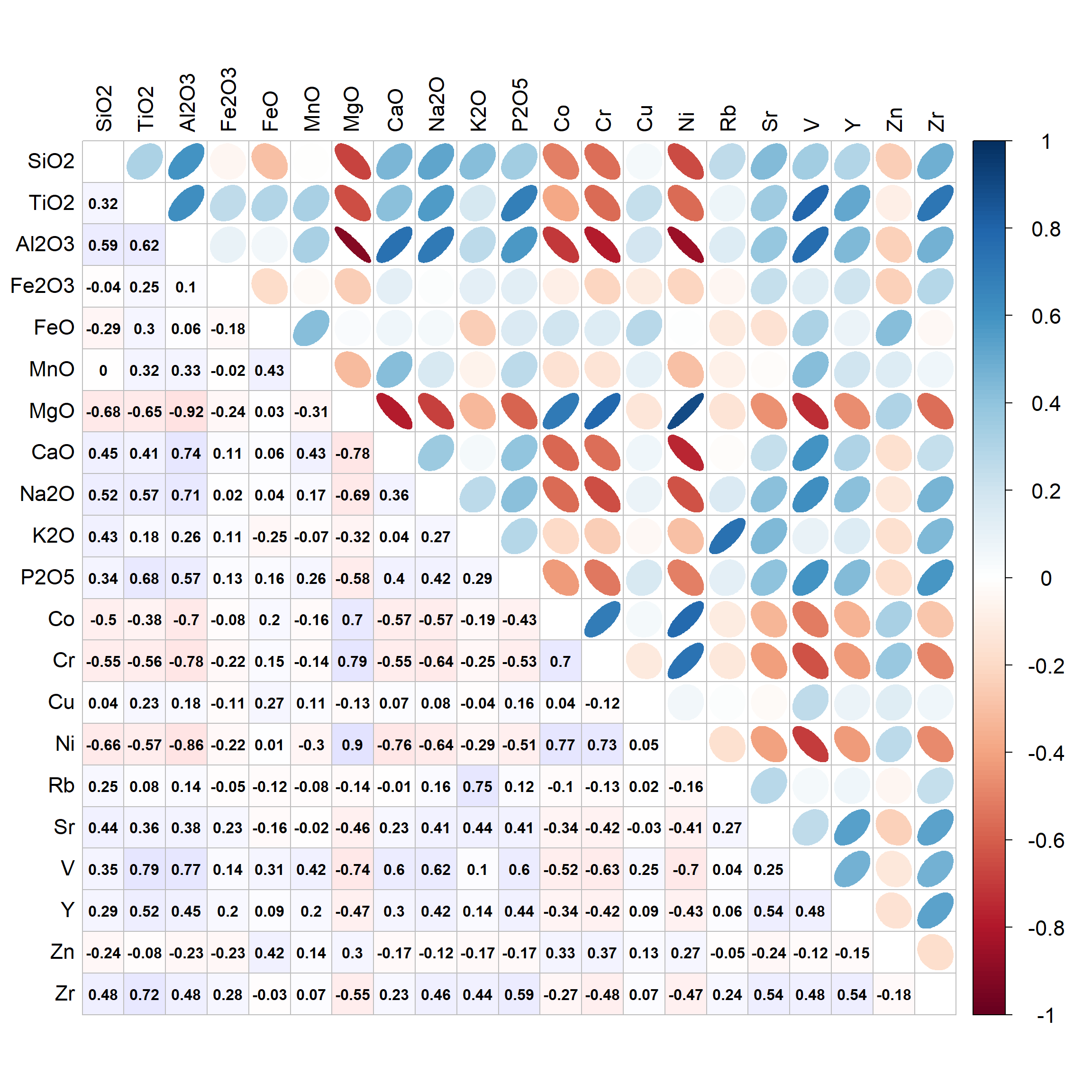
Figure 1: Correlation matrix for closed-set predictors (not part of LDA output)>
LDA on open (CLR) whole rock major element data
data0 <- Hallberg_clr
data0[,c(15:25,28:37)] <- scale(data0[,c(15:25,28:37)]) # scale just numeric variables
lda_rock_open <- lda(formula = Rock ~ SiO2 + TiO2 + Al2O3 + Fe2O3 + FeO + MnO +
                               MgO + CaO + Na2O + K2O + P2O5 + Co + Cr + Cu +
                               Ni + Rb + Sr + TiO2 + V + Y + Zn + Zr,
                    data = data0,
                    prior = as.numeric(summary(data0$Rock))/nrow(data0))
print(lda_rock_open)
## Call:
## lda(Rock ~ SiO2 + TiO2 + Al2O3 + Fe2O3 + FeO + MnO + MgO + CaO +
## Na2O + K2O + P2O5 + Co + Cr + Cu + Ni + Rb + Sr + TiO2 +
## V + Y + Zn + Zr, data = data0, prior = as.numeric(summary(data0$Rock))/nrow(data0))
##
## Prior probabilities of groups:
## Basalt Dolerite Gabbro High-Mg Basalt Peridotite Spinel Peridotite
## 0.572237960 0.082152975 0.019830028 0.243626062 0.073654391 0.008498584
##
## Group means:
## SiO2 TiO2 Al2O3 Fe2O3 FeO MnO MgO CaO
## Basalt -0.25738187 0.2537924 0.4391688 -0.05095198 -0.31451236 -0.20473569 -0.4997587 0.22117524
## Dolerite -0.44744406 0.3995203 0.3124530 -0.65188391 -0.04020638 -0.32690019 -0.3417888 0.06871215
## Gabbro -0.73856003 0.6268184 0.4980210 -0.77364397 -0.04090888 -0.20827176 -0.6409722 -0.04989445
## High-Mg Basalt 0.04139358 -0.3768292 -0.5781595 0.17599105 0.06554438 0.02869537 0.4862839 0.04587332
## Peridotite 2.40586837 -1.2318624 -1.7532776 0.74104059 2.10239359 1.82020929 2.5760285 -1.83933626
## Spinel Peridotite 1.34150366 -0.9347177 -1.9841498 0.07005191 1.56159769 0.83379111 2.1842575 -0.81438407
## Na2O K2O P2O5 Co Cr Cu Ni Rb Sr
## Basalt 0.4384678 0.21987167 0.4002674 -0.4237590 -0.4987620 0.08412522 -0.4535467 -0.04076464 0.3787489
## Dolerite 0.3278769 0.14481862 0.6579856 -0.4818491 -0.5237427 0.41970263 -0.4723105 0.09066789 0.1653297
## Gabbro 0.4570478 0.29204599 0.8366189 -0.7165812 -0.6691570 0.51172142 -0.6727888 0.16761638 0.0440467
## High-Mg Basalt -0.3145889 0.02023643 -0.6683486 0.3640927 0.7938929 -0.40704189 0.4003037 0.12161747 -0.4312253
## Peridotite -2.6333811 -1.79286121 -1.6153835 2.5653261 1.8182359 0.02413714 2.6339247 -0.21734714 -1.5805855
## Spinel Peridotite -1.9185672 -1.92802674 -2.1046561 2.1928540 1.6912115 0.54377178 2.3715978 -0.12543422 -1.1431906
## V Y Zn Zr
## Basalt 0.3514809 0.3641648 -0.2255523 0.3536939
## Dolerite 0.4385002 0.3361024 -0.1129799 0.2534661
## Gabbro 0.5247575 0.3886290 0.2333842 0.2550671
## High-Mg Basalt -0.4946752 -0.4070925 0.1464523 -0.3289291
## Peridotite -1.5608713 -1.8247550 1.1886606 -1.7881890
## Spinel Peridotite -1.4214092 -1.1916923 1.2347375 -1.9337810
##
## Coefficients of linear discriminants:
## LD1 LD2 LD3 LD4 LD5
## SiO2 0.311906556 0.475172430 1.06386434 -0.31153403 -0.49360643
## TiO2 -0.035043310 0.151688641 -0.14721971 -0.09186873 0.17887478
## Al2O3 -0.312637279 0.466394555 -0.14735485 -0.30383542 0.40628481
## Fe2O3 -0.022620301 -0.390680981 0.66513139 -0.12737824 0.29133594
## FeO -0.063901662 0.595404868 -0.15423496 -0.26329116 0.26140339
## MnO 0.232120983 0.273346069 0.18819409 -0.43680365 0.26962349
## MgO 0.531918843 -0.401806131 -2.67147472 -0.18459843 -1.74702057
## CaO -0.615973836 -0.613615069 -0.28059295 0.48378064 -0.31940725
## Na2O -0.738743065 -0.498253105 0.21204722 0.80358159 -0.17175823
## K2O 0.021600745 -0.380364118 0.01703155 -0.70089981 -0.31534337
## P2O5 -0.430115909 0.472152464 -0.32302277 -0.33080910 -0.19785901
## Co 0.443719497 -0.291897897 -0.23779641 0.39291494 -0.08560493
## Cr 0.306727775 -1.047240560 0.54144693 -0.76768593 0.46797732
## Cu -0.059583571 0.149775151 -0.12979112 0.14745878 0.01141351
## Ni 0.147582733 0.824302811 0.87784570 1.62502433 0.18782951
## Rb 0.002277406 0.308139649 -0.09488075 0.13556801 0.26716383
## Sr 0.483922453 0.689810105 0.01330317 0.34114182 -0.15189125
## V 0.023458566 0.001742575 0.06663428 0.07764911 -0.39425633
## Y -0.028468272 0.031123166 -0.15387790 0.34661178 0.12424677
## Zn -0.089890850 -0.073273061 0.06237525 -0.05846468 0.53558740
## Zr 0.097653277 -0.197155426 -0.06140115 -0.31397470 -0.61079156
##
## Proportion of trace:
## LD1 LD2 LD3 LD4 LD5
## 0.8494 0.1247 0.0173 0.0071 0.0015
cormat <- cor(data0[,c(15:25,28:37)])
cmx <- round(cormat,3) ; cmx[which(cmx>0.9999)] <- NA
corrplot(cmx, method="ellipse", type="upper", tl.col=1, tl.cex=1.4,
                   cl.cex=1.4, na.label = " ", tl.pos="lt")
corrplot(cmx, method="ellipse", type="lower", tl.col=1, addCoef.col=1,
         addgrid.col = "grey", na.label = " ", cl.pos="n", tl.pos="n", add=TRUE,
         col=colorRampPalette(c("#ffe0e0","white","#e0e0ff"))(200))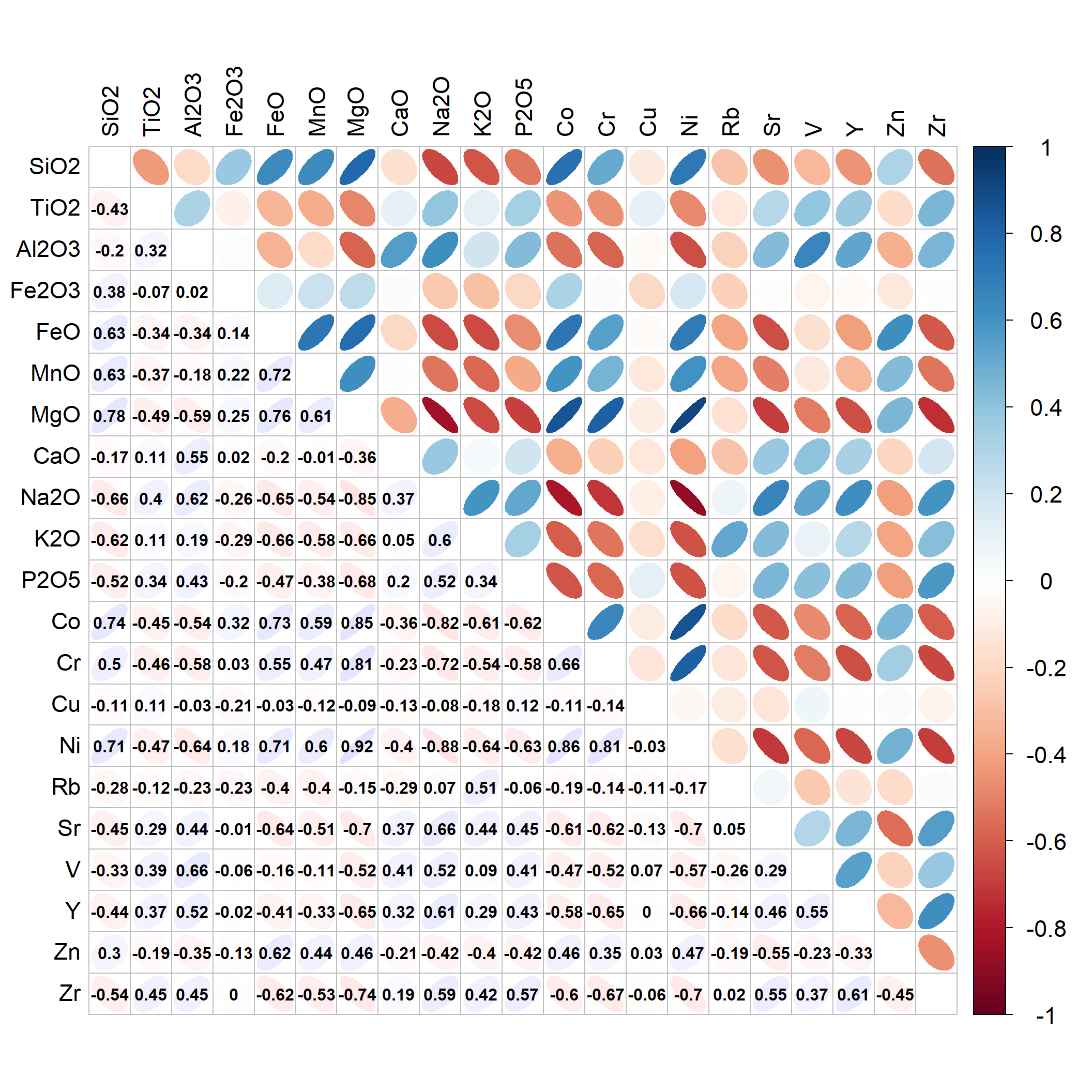
Figure 2: Correlation matrix for clr-transformed predictors (not part of LDA output)>
The LDA model specified and the prior probabilities are reported back to us in the output. The Group means sub-table in the output contains the centroids of the categories (5 classes, in our whole rock data) in the n-dimensional space defined by the n variables used for classification. The Coefficients of linear discriminants sub-table essentially defines the linear discriminant functions that separate our categories, since each function (LD1, LD2, etc.) is a linear combination of all the variables. Finally, the Proportion of trace sub-table gives the proportions of between-class variance that are explained by successive discriminant functions (e.g. for the open Hallberg rock data, LD1 explains 0.849 (85%) and LD2 explains 0.125 (12.5%) of variance between Rock type categories).
[Note: sometimes we cannot make an LDA model, because the predictors are collinear (highly correlated). We may be able to fix this by inspecting a correlation matrix for all the predictor variables, and removing one variable at a time from correlated pairs, then re-running the LDA procedure. By analogy with multiple linear regression, this would mean a Pearson's r ≥ 0.8.]
Visualising LDA separation
LDA histograms
We can plot the separation achieved by each linear discriminant (LD)
function by predicting the classification using the input data, then
using the ldahist() function (Venables and Ripley 2002). To
see the separation in another LDA dimension, we change the subscript in
the predClos$x[,1] option. Histograms (actually drawn with
custom code, enabling a plot with a side-by side comparison) are shown
in Figure 3.
predClos <- predict(lda_rock_clos, Hallberg[,c(15:25,28:37)])
predOpen <- predict(lda_rock_open, Hallberg[,c(15:25,28:37)])
LD1c <- data.frame(Rock=as.character(Hallberg$Rock),LD1=predClos$x[,1])
LD1c$Rock <- factor(LD1c$Rock, levels=levels(Hallberg$Rock))
par(mfcol = c(nlevels(LD1c$Rock),2), mar = c(1,2,1,1), oma = c(1,0,1,0),
    mgp = c(0.75,0.2,0), tcl=0.15)
for (i in 1:nlevels(LD1c$Rock)){
  with(subset(LD1c, subset=LD1c$Rock==levels(LD1c$Rock)[i]),
       hist(LD1, main = "", breaks = pretty(LD1c$LD1, n=20), col=5,
       xlim = c(min(LD1c$LD1, na.rm=T),max(LD1c$LD1, na.rm=T))))
  box()
  mtext(levels(LD1c$Rock)[i],3,-1.55,adj=0.505, cex = 0.85, font = 2, col=14)
  mtext(levels(LD1c$Rock)[i],3,-1.5, cex = 0.85, font = 2, col = 11)
  if(i==1) mtext("(a) Closed data", 3, 0.5, font=2, cex = 1.4, col = 11)
}

LD1o <- data.frame(Rock=as.character(Hallberg$Rock),LD1=predOpen$x[,1])
LD1o$Rock <- factor(LD1o$Rock, levels=levels(Hallberg$Rock))
for (i in 1:nlevels(LD1o$Rock)){
  with(subset(LD1o, subset=LD1o$Rock==levels(LD1o$Rock)[i]),
       hist(LD1, main = "", breaks = pretty(LD1o$LD1, n=20), col=4,
            xlim = c(min(LD1o$LD1, na.rm=T),max(LD1o$LD1, na.rm=T))))
  box()
  mtext(levels(LD1o$Rock)[i],3,-1.55, adj=0.505, cex = 0.85, font = 2, col=14)
  mtext(levels(LD1o$Rock)[i],3,-1.5, cex = 0.85, font = 2, col = 2)
  if(i==1) mtext("(b) Open data", 3, 0.5, font=2, cex = 1.4, col = 2)
}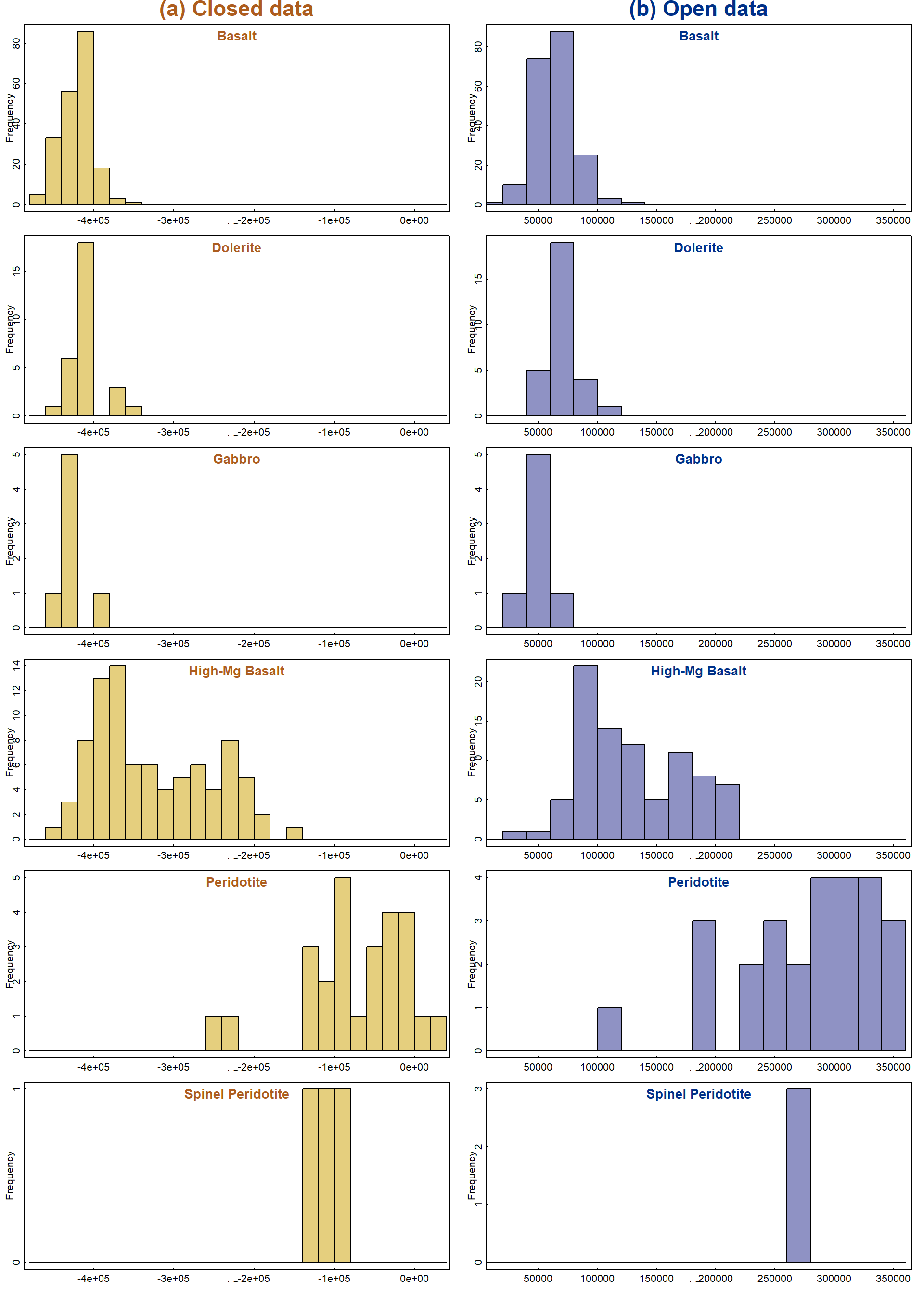
Figure 3: Histograms based on the first linear discriminant function for (a) closed and (b) open (CLR-transformed) whole-rock major element data.
The sets of histograms for closed and open data in Figure 3 both show some separation of categories, but with overlap. Of course this only shows the separation in one dimension, and two or more dimensions may be needed to achieve clear separation. We will make plots showing more than one LDA dimension later.
Partition plots
Another potentially useful way of showing separation of groups in LDA
is to use a partition plot, accessible using the
partimat() function from the klaR R package
(Weihs et al. 2005).
require(klaR)
par(mfrow = c(1,2),mar = c(3,3,1,1), mgp= c(1.3,0.2,0), tcl=0.2, font.lab=2)
with(Hallberg,
     drawparti(Rock, TiO2, Zr, method="lda",image.colors = c(10,7,14,13,2:3),
               xlab = expression(bold(paste(TiO[2]," (mg/kg)"))),
               ylab = expression(bold(paste(Zr," (mg/kg)"))))
     )
mtext("(a)", 3, -1.5, adj=0.05, font=2, cex = 1.2)
with(Hallberg_clr,
     drawparti(Rock, TiO2, Zr, method="lda",image.colors = c(10,7,14,13,2:3),
               xlab = expression(bold(paste(TiO[2]," (CLR-transformed)"))),
               ylab = expression(bold(paste(Zr," (CLR-transformed)"))))
     )
mtext("(b)", 3, -1.5, adj=0.95, font=2, cex = 1.2)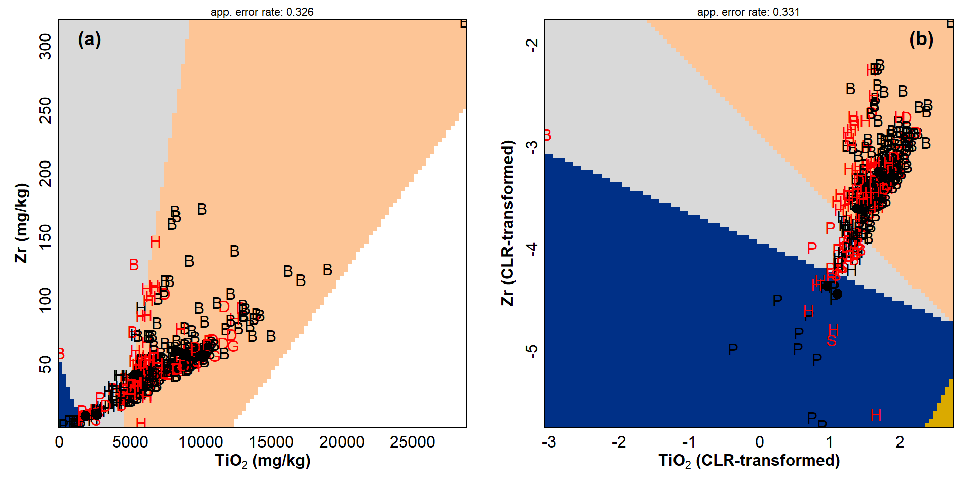
Figure 4: Partition plots for (a) closed and (b) open (CLR-transformed) whole rock major element data, based on the TiO₂ and Zr contents. Filled symbols are means in each category, with red letters showing apparently mis-classified observations.
Partition plots, such as those in Figure 4, are presented for single
pairwise combinations of the variables (in this example TiO2
and Zr) used to make the LDA model. We can make different plots by
specifying different variables in the drawparti() function.
Each such plot can be considered to be a different view of the data
(which of course has multiple dimensions). Coloured regions delineate
each classification area. Any observation that falls within a region is
predicted to be from a specific category, with apparent
mis-classification in a different color (but we usually need more than
two dimensions for correct classification). Each plot also includes the
apparent error rate for that view of the data.
Scatter Plots resembling biplots
Scatter-plots showing each variable and observation in linear discriminant dimensions, and grouped by category, are useful for visual assessment of how well the LDA model separates the observations.
par(mfrow = c(2,2), mar = c(3.5,3.5,1,1), mgp = c(1.5,0.3,0), tcl = 0.25,
    lend = "square", ljoin = "mitre", cex.main = 0.9, font.lab=2)
palette(c("black", viridis::viridis(6, alp=0.7, end=0.99), "gray","transparent"))
plot(lda_rock_clos$scaling[,1], lda_rock_clos$scaling[,2], type="n",
     xlim = c(-1,1), # ylim=c(-0.8,1.4),
     xlab="Linear Discriminant [1]", ylab="Linear Discriminant [2]",
     main="(a) Variable Coefficients [LD1, LD2]")
abline(v=0,col="grey",lty=2)
abline(h=0,col="grey",lty=2)
text(lda_rock_clos$scaling[,1],lda_rock_clos$scaling[,2],
     labels=names(Hallberg)[c(15:25,28:37)], pos = c(4,4,2,4,4,1,1,1,4,2,3),
     cex = 1.1, col = 2, offset = 0.2)
mtext("(a)", 3, -1.5, adj = 0.95, cex = 1.2, font = 2)

ldaPred_rock_clos <- predict(lda_rock_clos)

for(i in 1:NROW(lda_rock_clos$scaling)){
  arrows(0,0,lda_rock_clos$scaling[i,1],lda_rock_clos$scaling[i,2],
         length = 0.1, col = 8)
}

plot(ldaPred_rock_clos$x[,1], ldaPred_rock_clos$x[,2],
     bg=c(2:7)[Hallberg_clr$Rock],
     pch=c(21:25,21)[Hallberg_clr$Rock], lwd = 1, cex = 1.5,
  xlab="Linear Discriminant [1]", ylab="Linear Discriminant [2]",
  main="Predictions for Observations [LD1, LD2]")
abline(v=0,col="grey",lty=2)
abline(h=0,col="grey",lty=2)
# text(ldaPred_rock_clos$x[,1], ldaPred_rock_clos$x[,2],
#      labels=as.character(Hallberg$Rock), col=c(2,4,6,3,12)[Hallberg$Rock],
#      pos=1, offset=0.15, cex=0.65)
# legend("bottomright",legend=levels(Hallberg$Rock)[6:13],
#        ncol = 2, col=c(6:13), pch=c(5:12), pt.lwd = 2,
#        title=expression(bold("Rock Type")),
#        bty="n", inset=0.01,
#        pt.cex=c(1.8,1.8,2,2,1.3), cex=0.9)
mtext("(b)", 3, -1.5, adj = 0.95, cex = 1.2, font = 2)

plot(ldaPred_rock_clos$x[,1], ldaPred_rock_clos$x[,3],
     bg=c(2:7)[Hallberg_clr$Rock],
     pch=c(21:25,21)[Hallberg_clr$Rock], lwd = 1, cex = 1.5,
  xlab="Linear Discriminant [1]", ylab="Linear Discriminant [3]",
  main="Predictions for Observations [LD1, LD3]")
abline(v=0,col="grey",lty=2)
abline(h=0,col="grey",lty=2)
# text(ldaPred_rock_clos$x[,1], ldaPred_rock_clos$x[,3],
#      labels=Hallberg$Rock, col=c(1:13)[Hallberg$Rock],
#      pos=1, offset=0.15, cex=0.65)
mtext("(c)", 3, -1.5, adj = 0.05, cex = 1.2, font = 2)

plot(ldaPred_rock_clos$x[,2], ldaPred_rock_clos$x[,4],
     bg=c(2:7)[Hallberg_clr$Rock],
     pch=c(21:25,21)[Hallberg_clr$Rock], lwd = 1, cex = 1.5,
  xlab="Linear Discriminant [2]", ylab="Linear Discriminant [4]",
  main="Predictions for Observations [LD2, LD4]")
abline(v=0,col="grey",lty=2)
abline(h=0,col="grey",lty=2)
# text(ldaPred_rock_clos$x[,2], ldaPred_rock_clos$x[,4],
#      labels=Hallberg$Rock, col=c(2,4,6,3,12)[Hallberg$Rock],
#      pos=1, offset=0.15, cex=0.65)
mtext("(d)", 3, -1.5, adj=0.05, cex=1.2, font=2)
legend("bottomright",legend=levels(Hallberg$Rock), ncol=2, bty="n",
       inset=c(0.001,0.001), pt.bg=c(2:7), pch=c(21:25,21), pt.lwd=1,
    title="Rock Type in (b) - (d)", pt.cex=1.5, cex=1, y.intersp=1)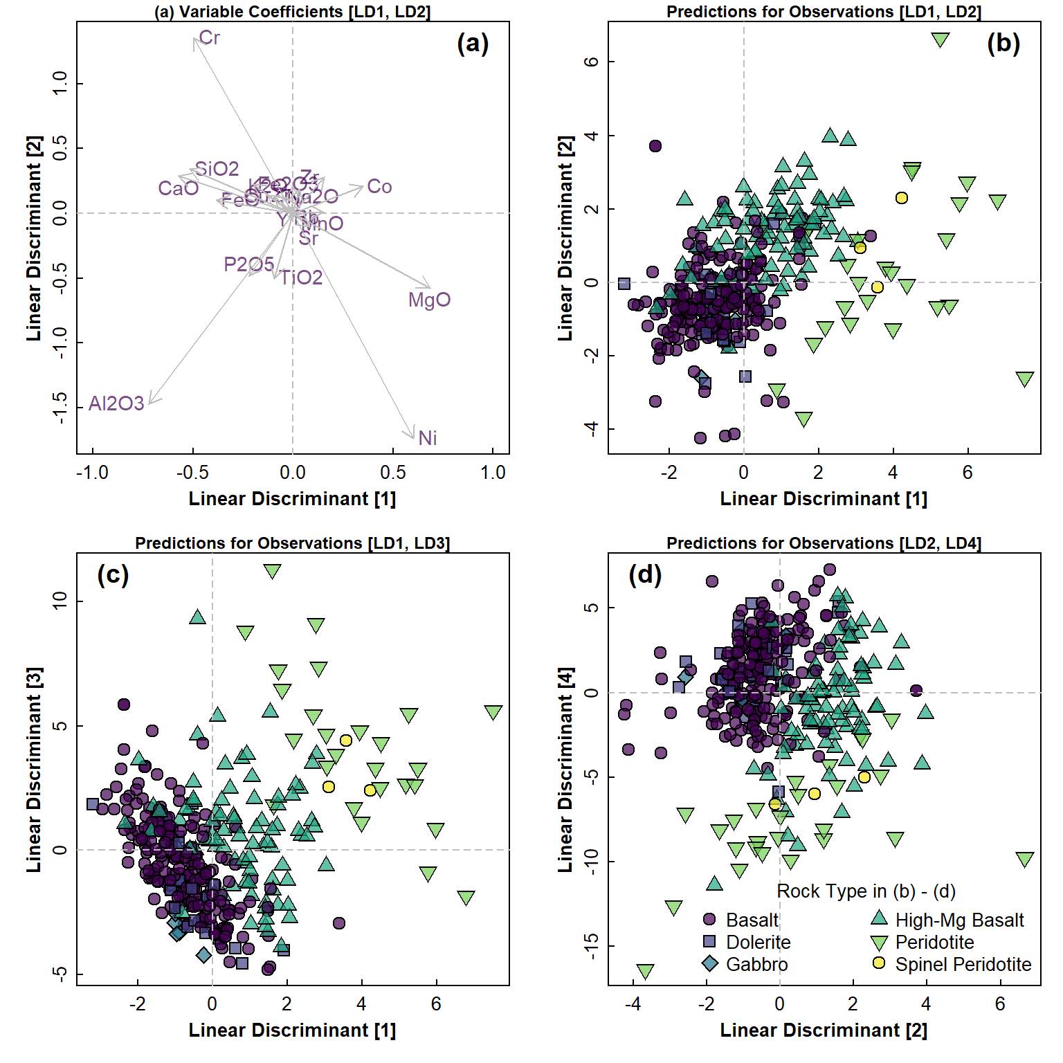
Figure 5: Linear discriminant analysis (LDA) plots for closed rock composition data: (a) variable coefficients in LD1-LD2 space, and predictions for observations in (b) LD1-LD2 space; (c) LD1-LD3 space; (d) LS2-LD4 space. Legend in (a) applies to plots in (b), (c), and (d).
par(mfrow = c(2,2), mar = c(3.5,3.5,1,1), mgp = c(1.5,0.3,0), tcl = 0.25,
    lend = "square", ljoin = "mitre", cex.main = 0.9, font.lab=2)
palette(c("black", viridis(6, alp=0.7, end=0.99), "gray","transparent","white"))
plot(lda_rock_open$scaling[,1], lda_rock_open$scaling[,2], type="n",
     xlim = c(-1,1),  ylim = c(-1.2,1),
     xlab="Linear Discriminant [1]", ylab="Linear Discriminant [2]",
     main="Variable Coefficients [LD1, LD2]")
abline(v=0,col="grey",lty=2); abline(h=0,col="grey",lty=2)
text(lda_rock_open$scaling[,1]*1.1, lda_rock_open$scaling[,2]*1.1,
     labels=names(Hallberg_clr)[c(15:25,28:37)],
     cex = 1.1, col = 3, offset=0.2, font=2)
for(i in 1:NROW(lda_rock_open$scaling)){
  arrows(0,0,lda_rock_open$scaling[i,1], lda_rock_open$scaling[i,2],
         length = 0.1, col = 8) }
mtext("(a)", 3, -1.5, adj = 0.05, cex = 1.2, font = 2)

ldaPred_rock_open <- predict(lda_rock_open)

plot(ldaPred_rock_open$x[,1], ldaPred_rock_open$x[,2],
     col="#000000a0",bg=c(2:7)[ldaPred_rock_open$class],
     pch=c(21:25,21)[ldaPred_rock_open$class], lwd=1, cex = 1.5,
     main="Predictions for Observations [LD1, LD2]",
     xlab="Linear Discriminant [1]", ylab="Linear Discriminant [2]")
points(ldaPred_rock_open$x[ldaPred_rock_open$class==data0$Rock,1],
       ldaPred_rock_open$x[ldaPred_rock_open$class==data0$Rock,2],
       pch=21, cex=0.5, col="#ffffffa0", bg="#000000c0")
abline(v=0,col="grey",lty=2); abline(h=0,col="grey",lty=2)
mtext("(b)", 3, -1.5, adj = 0.05, cex = 1.2, font = 2)
legend("bottomright", ncol = 1, bty="n", cex=0.85, title="Rock Type in (b)-(d)",
       legend=c(substr(levels(ldaPred_rock_open$class),1,7),"dots = correct"),
       pt.cex=c(rep(1.5,6),0.5), pt.bg=c(2:7,"#000000c0"), col=c(rep("#000000a0",6),10),
       pch=c(21:25,21,21), pt.lwd=1, box.col="grey90", y.intersp=0.95, box.lwd=2)

plot(ldaPred_rock_open$x[,1], ldaPred_rock_open$x[,3],
     bg=c(2:7)[ldaPred_rock_open$class],
     pch=c(21:25,21)[ldaPred_rock_open$class], lwd=1, cex = 1.5,
     main="Predictions for Observations [LD1, LD3]",
     xlab="Linear Discriminant [1]", ylab="Linear Discriminant [3]")
points(ldaPred_rock_open$x[ldaPred_rock_open$class==data0$Rock,1],
       ldaPred_rock_open$x[ldaPred_rock_open$class==data0$Rock,3],
       pch=21, cex=0.5, col="#ffffffa0", bg="#000000c0")
abline(v=0,col="grey",lty=2); abline(h=0,col="grey",lty=2)
mtext("(c)", 3, -1.5, adj = 0.05, cex = 1.2, font = 2)

plot(ldaPred_rock_open$x[,2], ldaPred_rock_open$x[,4],
     bg=c(2:7)[ldaPred_rock_open$class],
     pch=c(21:25,21)[ldaPred_rock_open$class], lwd=1, cex = 1.5,
     main="Predictions for Observations [LD2, LD4]",
     xlab="Linear Discriminant [2]", ylab="Linear Discriminant [4]")
points(ldaPred_rock_open$x[ldaPred_rock_open$class==data0$Rock,2],
       ldaPred_rock_open$x[ldaPred_rock_open$class==data0$Rock,4],
       pch=21, cex=0.5, col="#ffffffa0", bg="#000000c0")
abline(v=0,col="grey",lty=2); abline(h=0,col="grey",lty=2)
mtext("(d)", 3, -1.5, adj = 0.95, cex = 1.2, font = 2)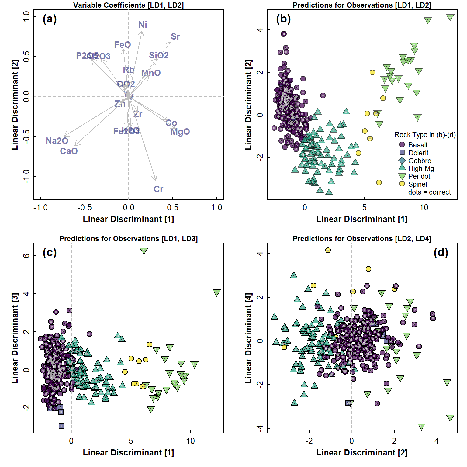
Figure 6: Linear discriminant analysis (LDA) plots for open (CLR-transformed) rock composition data: (a) variable coefficients in LD1-LD2 space, and predictions for observations (showing correct classes) in (b) LD1-LD2 space; (c) LD1-LD3 space; (d) LS2-LD3 space. Legend in (a) applies to plots (b), (c), and (d).
From the plots in Figure 5 and Figure 6, we can see that the LDA models obtained are certainly able to separate observations by the selected factor. Firstly, however, there is a lot of clustering of the predictor variables in Figure 5(a), which may relate to spurious relationships between variables caused by compositional closure. This clustering is not so pronounced in Figure 6(a), since the closure has been removed by CLR-transformation.
Out of the combinations of LDA dimensions selected, the best separation is with LD2 vs. LD1, which is not surprising since these dimensions together account for about 95% of the between-groups variance – for both closed and open data. There is a lot of apparent overlap, but we can not see the true separation in only 2 dimensions. The LDA performed on open data may result in slightly clearer separation of samples by Rock category than LDA using closed data, but without a multidimensional view this is also hard to be sure about.
Inspecting the agreement between actual and predicted categories in LDA
To do this easily we just make an R data frame with columns for the actual categories (from the original data frame) and the predicted categories (from the prediction objects we just made). We add a column telling us if these two columns match in each row (which we can see easily, but we use this column to calculate a numerical prediction accuracy).
We need to make objects containing the LDA predictions:
The code below uses the head() function to inspect the
first few rows of each comparison, but we could easily look at the whole
comparison data frames using print().
closComp <- data.frame(Actual = as.character(Hallberg$Rock),
                       Predicted = as.character(ldaPred_rock_clos$class))
closComp$test <- as.character(Hallberg_clr$Rock) ==
  as.character(ldaPred_rock_clos$class)
k = length(which(closComp$test == TRUE))
cat("Predictions by LDA using closed data:",k,"out of",NROW(Hallberg_clr),
    "=",paste0(round(100*k/NROW(Hallberg_clr),1),"% correct\n"))
head(closComp, n = 10)

openComp <- data.frame(Actual = as.character(Hallberg_clr$Rock),
                       Predicted = as.character(ldaPred_rock_open$class))
openComp$test <- as.character(Hallberg_clr$Rock) ==
  as.character(ldaPred_rock_open$class)
k = length(which(openComp$test == TRUE))
cat("\nPredictions by LDA using open data:",k,"out of",NROW(Hallberg_clr),
    "=",paste0(round(100*k/NROW(Hallberg_clr),1),"% correct\n"))
head(openComp, n = 10)
## Predictions by LDA using closed data: 238 out of 353 = 67.4% correct
## Actual Predicted test
## 1 Basalt Basalt TRUE
## 2 Basalt Basalt TRUE
## 3 Gabbro Dolerite FALSE
## 4 Basalt Basalt TRUE
## 5 Basalt Dolerite FALSE
## 6 Basalt Basalt TRUE
## 7 Basalt Basalt TRUE
## 8 Basalt Basalt TRUE
## 9 High-Mg Basalt Basalt FALSE
## 10 Dolerite Dolerite TRUE
##
## Predictions by LDA using open data: 295 out of 353 = 83.6% correct
## Actual Predicted test
## 1 Basalt Basalt TRUE
## 2 Basalt Dolerite FALSE
## 3 Gabbro Basalt FALSE
## 4 Basalt Basalt TRUE
## 5 Basalt Basalt TRUE
## 6 Basalt Basalt TRUE
## 7 Basalt Basalt TRUE
## 8 Basalt Basalt TRUE
## 9 High-Mg Basalt High-Mg Basalt TRUE
## 10 Dolerite Basalt FALSEFor this dataset, it seems as though LDA using open data is better at predicting the Rock category for each observation. In the output above, Basalt is mis-identified as Dolerite (which might make sense given the expected compositional similarity; simplistically, dolerite is a more coarse-grained version of basalt).
This kind of comparison is not very rigorous, and nor does it address the reason we might perform a supervised classification like LDA – to use data to predict unknown categories. The ability of LDA to predict unknown categories can be addressed by validation procedures, such as the one we investigate below.
Assessment of LDA prediction using a training-validation method
One way that we can get a better idea about the usefulness of our classification models is to perform some validation. This involves 'training' the model on a subset of our data, and trying to predict the category of a different subset using the training model.
This can be done quite simply, by including the
CV = TRUE option in the lda() function, which
implements 'leave one out cross validation'. Simply stated, this omits
one observation at a time, running the LDA on the remaining data each
time, and predicting the probability of the missed observation being in
each category (the posterior probabilities). [Each observation
is assigned to the category with the greatest posterior
probability.]
# leave-one-out cross validation for LDA
data0 <- Hallberg_clr
data0[,c(15:25,28:37)] <- scale(data0[,c(15:25,28:37)]) # scale just numeric variables
lda_rock_open <- lda(formula = Rock ~ SiO2 + TiO2 + Al2O3 + Fe2O3 + FeO + MnO +
                               MgO + CaO + Na2O + K2O + P2O5 + Co + Cr + Cu +
                               Ni + Rb + Sr + TiO2 + V + Y + Zn + Zr,
                     data = data0,
                     prior = as.numeric(summary(data0$Rock))/nrow(data0),
                     CV=TRUE)
preds <- apply(lda_rock_open$posterior, MARGIN = 1,
      FUN = function(x){levels(lda_rock_open$class)[which(x==max(x, na.rm=TRUE))]})
obsvs <- data0$Rock
matches <- data.frame(Pred_class=preds, Actual_class=obsvs, Match=preds==obsvs)
flextable(matches[1:20,]) |> bold(part="header") |> width(width=c(4.8,2.8,3.8), unit="cm") |>
  set_header_labels(Pred_class="Predicted class", Actual_class="Actual class",
                    Match="Is LDA correct?") |> padding(padding=0.5,part="all") |>
set_caption(caption="Table 2: Matches between LDA model and actual data based on CLR-transformed major element concentrations in the whole rock dataset compiled by Hallberg (2006). Only the first 20 observations are shown.")Predicted class | Actual class | Is LDA correct? |
|---|---|---|
Basalt | Basalt | true |
Dolerite | Basalt | false |
Basalt | Gabbro | false |
Basalt | Basalt | true |
Basalt | Basalt | true |
Basalt | Basalt | true |
Basalt | Basalt | true |
Basalt | Basalt | true |
High-Mg Basalt | High-Mg Basalt | true |
Basalt | Dolerite | false |
Basalt | Gabbro | false |
Basalt | Basalt | true |
Peridotite | Peridotite | true |
Spinel Peridotite | Peridotite | false |
Basalt | Basalt | true |
Peridotite | Peridotite | true |
Spinel Peridotite | Peridotite | false |
Peridotite | Peridotite | true |
Basalt | Basalt | true |
Basalt | Basalt | true |
Below we use a related method, using training and validation subsets of our data. The idea here is that we divide the dataset into two (the code below splits the data in half, but other splits could be used, e.g. 0.75:0.25). The first subset of the data is used to generate an LDA model (i.e. a set of linear discriminant functions), which are then used to try and predict the categories in the other subset. We choose the observations making up each subset randomly. Of course, this could give us unreliable results if the random selection happens to be somehow unbalanced, so we repeat the training-validation process many times to calculate an average prediction rate.
One glitch that can happen is that in selecting a random subset of the data, the subset may not include any samples from one or more categories. This problem is more likely if our data have some categories having relatively few observations. The code below applies an 'error-catching' condition before running the training LDA, which is that all categories in a random subset need to be populated.
n0 <- 200 # number of iterations
ftrain <- 0.5 # proportion of observations in training set
results <- data.frame(
  Rep = rep(NA, n0),
  matches = rep(NA, n0),
  non_matches = rep(NA, n0),
  success = rep(NA, n0))
train <- sample(1:NROW(Hallberg), round(NROW(Hallberg) * ftrain,0))
# make vector of individual category non-matches
matchByClass <-
  data.frame(Match1 = rep(0,nlevels(Hallberg$Rock[train])))
rownames(matchByClass) <- levels(ldaPred_rock_clos$class)
fMatchXClass <-
  data.frame(PctMch1 = rep(0,nlevels(Hallberg$Rock[train])))
rownames(fMatchXClass) <- levels(ldaPred_rock_clos$class)
# make vector of cumulative category counts in Hallberg[-train] iterations
cc0 <- rep(0,nlevels(Hallberg$Rock))
isOK <- 0 ; i <- 2

for (i in 1:n0) {
  train <- sample(1:NROW(Hallberg), round(NROW(Hallberg) * ftrain,0))
      # set condition requiring all categories to be populated
      if (is.na(match(NA,tapply(Hallberg[train,]$SiO2,
                      Hallberg[train,]$Rock, sd, na.rm=T))) == TRUE) {
          lda_Rock_train <- lda(formula = Rock ~ SiO2 + TiO2 + Al2O3 + Fe2O3 + FeO + MnO +
                               MgO + CaO + Na2O + K2O + P2O5 + Co + Cr + Cu +
                               Ni + Rb + Sr + TiO2 + V + Y + Zn + Zr,
                          data = Hallberg[train,],
                          prior=as.numeric(summary(Hallberg$Rock[train]))/
                            nrow(Hallberg[train,]))
          ldaPred_rock_clos <- predict(lda_Rock_train, Hallberg[-train,])
          isOK <- isOK + 1
        }

  k=0               # number of matches
  m0 <-             # vector of individual category matches
    as.matrix(rep(0,nlevels(Hallberg$Rock[train])))
  rownames(m0) <- levels(Hallberg$Rock)
  m1 <-             # vector of fractional category matches
    as.matrix(rep(0,nlevels(Hallberg$Rock[train])))
  rownames(m1) <- levels(Hallberg$Rock)
  for (jM in 1:NROW(Hallberg[-train,])) {
    for (jS in 1:nlevels(ldaPred_rock_clos$class)) {
      if((ldaPred_rock_clos$class[jM] == levels(ldaPred_rock_clos$class)[jS]) &
         (Hallberg$Rock[-train][jM] == levels(ldaPred_rock_clos$class)[jS]) )
        m0[jS] = m0[jS] + 1
      else  m0[jS] = m0[jS]
    }
    k = sum(m0)
  }
  cc0 <- cc0 + as.numeric(summary(Hallberg$Rock[-train]))
  m1 <- round(100*m0/as.numeric(summary(Hallberg$Rock[-train])),1)
  matchByClass[,paste0("Match",i)] <- m0
  fMatchXClass[,paste0("PctMch",i)] <- m1
  # output to results data frame: iteration, matches, non-matches, proportion matched
  results[i,] <- c(i, k, NROW(Hallberg[-train,])-k,
                   signif(k/NROW(Hallberg[-train,]),3))
}
# Output code block
cat(paste("[Based on", n0, "random subsets of",paste0(100*ftrain,"%"),
          "of the dataset to train LDA model\n",
     "      to predict remaining observations]\n"))
  cat("Number of obs. in random subsets =",NROW(train),
      " (predicting",NROW(Hallberg)-NROW(train),"samples)\n")
  print(numSummary(results[,2:4], statistics=c("mean","sd"))$table)
  ns0 <- numSummary(results$success)
  t0 <- t.test(results$success)
  cat(rep("-\u2013-",24),
      "\nStat. summary for 'success':\nMean = ",round(ns0$table[1],4),
      ", sd = ",round(ns0$table[2],4),
      ", 95% confidence interval = (",
      signif(t0$conf.int[1],3),", ",signif(t0$conf.int[2],4),
      ") (after ",i," reps)\n", sep="")
  cat(n0-isOK,"iterations 'failed' due to randomisation missing a category\n\n")
  cat("Fraction of matches by category over ALL iterations:\n")
  summCats <- data.frame(
    Rock_Type = row.names(matchByClass),
    Total_Matched = rowSums(matchByClass),
    Actual = cc0,
    Percent_Matched = paste0(round(100*(rowSums(matchByClass)/cc0),1),"%"),
    row.names = NULL)
  print(summCats)
## [Based on 200 random subsets of 50% of the dataset to train LDA model
## to predict remaining observations]
## Number of obs. in random subsets = 176 (predicting 177 samples)
## mean sd
## matches 108.95500 25.4665605
## non_matches 68.04500 25.4665605
## success 0.61557 0.1438693
## -–--–--–--–--–--–--–--–--–--–--–--–--–--–--–--–--–--–--–--–--–--–--–--–-
## Stat. summary for 'success':
## Mean = 0.6156, sd = 0.1439, 95% confidence interval = (0.596, 0.6356) (after 200 reps)
## 106 iterations 'failed' due to randomisation missing a category
##
## Fraction of matches by category over ALL iterations:
## Rock_Type Total_Matched Actual Percent_Matched
## 1 Basalt 16237 20229 80.3%
## 2 Dolerite 200 2873 7%
## 3 Gabbro 13 675 1.9%
## 4 High-Mg Basalt 4355 8689 50.1%
## 5 Peridotite 937 2616 35.8%
## 6 Spinel Peridotite 49 318 15.4%The number of iterations makes some difference (Figure 5)!
Based on Figure 7, it looks like we should run at least 50-100 iterations to get a reasonable idea of how well our LDA model performs. More iterations are better, but it depends how long you want the run-time to be!
par(mar = c(3,3,1,1), mgp = c(1.5,0.2,0), tcl = 0.25, font.lab = 2)
plot(c(10,20,50,100,200,500,1000),c(0.5572,0.5986,0.5848,0.5847,0.5837,0.581,0.582),
     pch=19, cex = 1.2, log = "x", xlim = c(7,1400), ylim = c(0.45,0.65),
     xlab = "Number of iterations", ylab = "Mean accuracy \u00B1 95% CI")
arrows(c(10,20,50,100,200,500,1000),c(0.49,0.58,0.572,0.574,0.577,0.576,0.579),
       c(10,20,50,100,200,500,1000),c(0.624,0.617,0.598,0.595,0.591,0.586,0.585),
       angle = 90, length = 0.1, code = 3)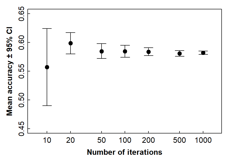
Figure 7: Accuracy (shown by 95 percent CI error bars) as a function of number of train-validate iterations for an LDA model using closed whole-rock composition data.
We can run a similar validation process for the CLR-transformed data
(we don't show the code, as it's effectively identical to
the code for validation of LDA for closed data, but with references to
Hallberg replaced with Hallberg_clr).
## [Based on 200 random subsets of 50% of the dataset to train LDA model
##        to predict remaining observations]
## Number of obs. in random subsets = 176  (predicting 177 samples)
##                  mean         sd
## matches     112.69500 26.3938468
## non_matches  64.30500 26.3938468
## success       0.63667  0.1491417
## -–--–--–--–--–--–--–--–--–--–--–--–--–--–--–--–--–--–--–--–--–--–--–--–-
## Stat. summary for 'success':
## Mean = 0.6367, sd = 0.1491, 95% confidence interval = (0.616, 0.6575) (after 200 reps)
## 98 iterations 'failed' due to randomisation missing a category
##
## Fraction of matches by category over ALL iterations:
##           Rock_Type Total_Matched Actual Percent_Matched
## 1            Basalt         16481  20224           81.5%
## 2          Dolerite           240   2893            8.3%
## 3            Gabbro             0    672              0%
## 4    High-Mg Basalt          4665   8681           53.7%
## 5        Peridotite          1107   2643           41.9%
## 6 Spinel Peridotite            46    287             16%
If we compare the validation output for the open data with the results for closed data, we see slightly better overall accuracy for open data. Both closed and open data generated successful predictions > 60% of the time, with a slightly greater standard deviation for LDA based on open data.
There were small differences (in this validation exercise), between closed and open data, in the ability of LDA to predict specific categories. Open-data LDA seemed better at predicting most categories; neither open- or closed-data LDA was good at predicting if a rock was Gabbro.
An issue that we haven't considered yet is whether all the variables
we used for prediction are necessary to discriminate the categories in
our data (some are collinear, based on Figure 2). The R package
klaR (Weihs et al. 2005) includes the
stepclass() function, which enables us to refine an LDA
model, using a procedure similar to stepwise selection of predictors in
multiple regression. The next chunk of code implements this
approach.
minimp <- c(0.0005,0.001,0.002,0.003,0.005,0.01) ; j <- 2
# for(j in 1:length(minimp)){
  stepwise.lda <- stepclass(formula = Rock ~ SiO2 + TiO2 + Al2O3 + Fe2O3 + FeO + MnO +
                               MgO + CaO + Na2O + K2O + P2O5 + Co + Cr + Cu +
                               Ni + Rb + Sr + TiO2 + V + Y + Zn + Zr,
                            data = data0, output=TRUE,
                            prior=as.numeric(summary(data0$Rock))/nrow(data0),
                            method="lda", improvement=minimp[j],
                            direction="backward", criterion="AS")
  # }
  cat("Stepwise model: ",deparse(stepwise.lda$formula)) # cleaner output
## abiltity to seperate: 0.78948; starting variables (21): SiO2, TiO2, Al2O3, Fe2O3, FeO, MnO, MgO, CaO, Na2O, K2O, P2O5, Co, Cr, Cu, Ni, Rb, Sr, V, Y, Zn, Zr
## abiltity to seperate: 0.78948; out: "SiO2"; variables (20): TiO2, Al2O3, Fe2O3, FeO, MnO, MgO, CaO, Na2O, K2O, P2O5, Co, Cr, Cu, Ni, Rb, Sr, V, Y, Zn, Zr
## abiltity to seperate: 0.79557; out: "Fe2O3"; variables (19): TiO2, Al2O3, FeO, MnO, MgO, CaO, Na2O, K2O, P2O5, Co, Cr, Cu, Ni, Rb, Sr, V, Y, Zn, Zr
## abiltity to seperate: 0.79595; out: "Y"; variables (18): TiO2, Al2O3, FeO, MnO, MgO, CaO, Na2O, K2O, P2O5, Co, Cr, Cu, Ni, Rb, Sr, V, Zn, Zr
## abiltity to seperate: 0.79736; out: "Co"; variables (17): TiO2, Al2O3, FeO, MnO, MgO, CaO, Na2O, K2O, P2O5, Cr, Cu, Ni, Rb, Sr, V, Zn, Zr
##
## hr.elapsed min.elapsed sec.elapsed
## 0.0 0.0 5.5
##
## Stepwise model: Rock ~ TiO2 + Al2O3 + FeO + MnO + MgO + CaO + Na2O + K2O + P2O5 + Cr + Cu + Ni + Rb + Sr + V + Zn + Zr
The ‘full’ LDA model had 21 predictors, but the stepwise model
retains fewer predictors, depending on individual code runs and/or
choice of options (see below). For example, the stepclass()
function does not remove the same variable first every time, using
"backward" predictor selection (we can change this to
"both", but "backward" makes sense if we start
with a ‘full’ LDA model).
If we run the code above repeatedly, we get different results. We
also get different results if we change the options in
stepclass() (for example, the default tolerance specified
by improvement= is 0.05, which I've found to not be
sensitive enough). We can also specify different criteria to optimise;
the code uses criterion="AS", which is ‘ability to
separate’, but we can choose others, such as correctness rate
("CR", the default), accuracy "AC", or
confidence "CF". For full details run
?klaR::stepclass. If you copy the code above, uncomment the
lines beginning with #, and run, you can see what the
effect of changing the improvement tolerance is.
Overall, Linear Discriminant Analysis offers a relatively simple way to predict pre-existing categories in a dataset based on multiple numeric variables. If we dont know what the categories should be, we would need to use a different type of multivariate procedure, such as one of the cluster analysis methods.
References
Hallberg, J.A. (2006). Greenstone chemistry from the Yilgarn Craton. Dataset ANZWA1220000718, Department of Energy, Mines, Industry Regulation and Safety, East Perth, Western Australia https://catalogue.data.wa.gov.au/dataset/hallberg-geochemistry.
Reimann, C., Filzmoser, P., Garrett, R. G., and Dutter, R. (2008). Statistical Data Analysis Explained: Applied Environmental Statistics with R (First ed.). John Wiley & Sons, Chichester, UK.
Venables, W. N. and Ripley, B. D. (2002) Modern Applied
Statistics with S (MASS). Fourth Edition. Springer,
New York. ISBN 0-387-95457-0 http://www.stats.ox.ac.uk/pub/MASS4/.
Weihs, C., Ligges, U., Luebke, K. and Raabe, N. (2005).
klaR – Analyzing German Business Cycles.
In Baier, D., Decker, R. and Schmidt-Thieme, L. (eds.).
Data Analysis and Decision Support, 335-343, Springer-Verlag,
Berlin.
CC-BY-SA • All content by Ratey-AtUWA. My employer does not necessarily know about or endorse the content of this website.
Created with rmarkdown in RStudio. Currently using the free yeti theme from Bootswatch.