Using R for soil profile diagrams

Material to support teaching in Environmental Science at The University of Western Australia

Units ENVT3361, ENVT4461, and ENVT5503

We're going to illustrate some more methods for drawing depth profiles and their trends using some real sediment core data. As before, you would need to adapt the R code examples to match your dataset and variable names.

First we read in a file and do some corrections of the data:

git <- 
  "https://raw.githubusercontent.com/Ratey-AtUWA/Learn-R-web/refs/heads/main/"
afs25 <- read.csv(paste0(git,"afs25.csv"), stringsAsFactors = TRUE)
afs25$Unit <- as.factor(afs25$Unit)
afs25$Group <- as.factor(afs25$Group)
afs25$SampleID <- as.character(afs25$SampleID)
afs25$Notes <- as.character(afs25$Notes)

Boxplots in depth categories

This may be a useful approach if we want to summarise depth trends across a site or stratum, especially if profiles are of different depths (i.e. under-representation of greater depths).

We need the rcompanion package for the fullPTable() function, the multcompView package for the multcompLetters() function, and the TeachingDemos package for the shadowtext() function.

afs25$DepthF <- cut(afs25$Depth_mean, breaks=c(0,10,20,30,100), 
                    labels = c("0-10cm","10-20cm","20-30cm",">30cm"))
par(mfrow=c(1,1), mar=c(1,5,3,1), mgp=c(1.6,0.4,0), tcl=-0.2, lend="square",
    font.lab=2)
palette(c("black","blue3","navy","red3","#ffa00040","white","transparent"))
with(afs25, boxplot(log10(Cu) ~ DepthF, horizontal=T, boxwex=1, ylab="", 
                    xaxt="n", xlab="", xaxs="i", col=5, 
                    cex=1.2, xlim=c(4.3,0.7), las=1, xaxt="n"))
abline(h=seq(1.5,3.5), lty=2, col="#00000040")
axis(3, at=log10(c(1,2,5,10,20,50,100,200,500)), 
          labels=c(1,2,5,10,20,50,100,200,500))
mtext("Cu (mg/kg)", side=3, line=1.6, font=2)
mtext("Depth Range", side=2, line=4, font=2)
meanz <- with(afs25, tapply(log10(Cu), DepthF, mean, na.rm=T))
points(meanz, 1:nlevels(afs25$DepthF), pch=3, col=6, lwd=4)
points(meanz, 1:nlevels(afs25$DepthF), pch=3, col=2, lwd=2)
kwt <- kruskal.test(Cu~DepthF, data=afs25)
pwt <- with(afs25, pairwise.wilcox.test(Cu, DepthF))
fpt <- fullPTable(pwt$p.value)
cld <- multcompLetters(fpt)
shadowtext(meanz, 1:nlevels(afs25$DepthF), labels=signif(meanz,3), 
           font=2, family="sans", pos=1, col=3, bg=6,r=0.2)
shadowtext(meanz, 1:nlevels(afs25$DepthF), labels=cld[[2]], 
           font=3, family="serif", pos=3, col=2, bg=6, r=0.2)
text(max(log10(afs25$Cu), na.rm=T), 4.3,
     pos=2, col=3, labels=paste("Kruskal-Wallis p =",signif(kwt$p.value,2)))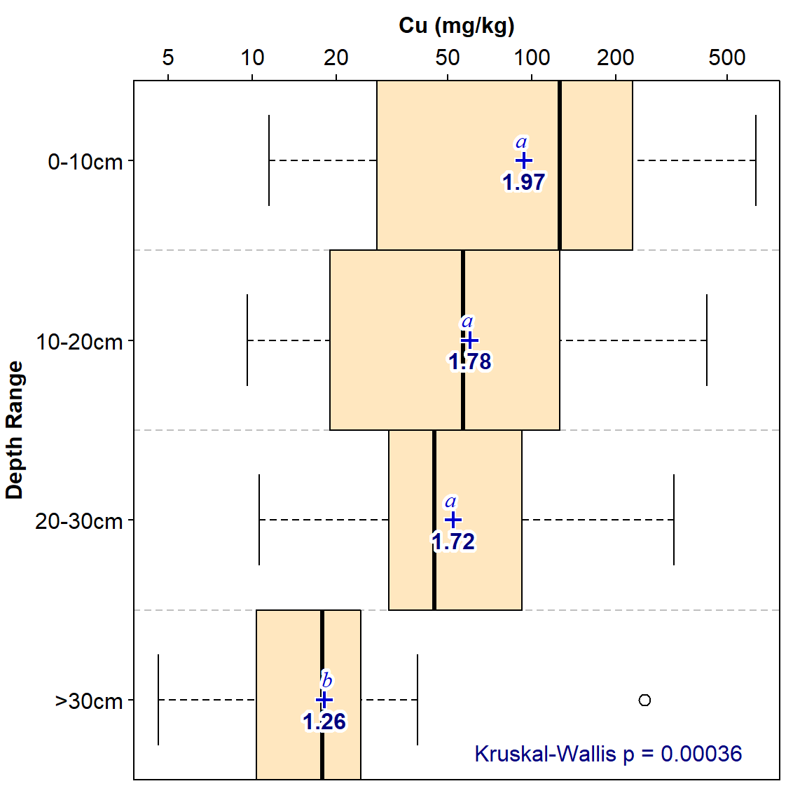

Figure 1: Depth profile of copper in multiple sediment cores, shown as boxplots in depth categories. Mean values are shown as blue '+' symbols; the letters above symbols differ if pairwise Wilcoxon test comparisons are significant (p ≤ 0.05). Bold numbers under '+' symbols are mean values.

Variable as a linear function of depth – many profiles

This may be another useful way to summarise depth trends, again especially if profiles are of different depths (i.e. not all depths are equally represented).

We do everything in base-R without additional packages.

par(mfrow=c(1,1), mar=c(1,3,3,1), mgp=c(1.6,0.4,0), tcl=-0.2, lend="square",
    font.lab=2)
palette(c("black","blue3","red3","#ff000040","#ffffffc0","transparent"))
with(afs25, plot(log10(Cu), Depth_mean, type="n", ylab="",
                 xaxt="n", xlab="", yaxs="i", cex=1.2, 
                 xlim=log10(c(3,640)), ylim=c(70,0), 
                 las=1, xaxt="n"))
abline(h=seq(10,60,10), lty=2, col="#00000040")
axis(3, at=log10(c(1,2,5,10,20,50,100,200,500)), 
          labels=c(1,2,5,10,20,50,100,200,500))
mtext("Cu (mg/kg)", side=3, line=1.6, font=2)
mtext("Depth (cm)", side=2, line=1.6, font=2)
lm0 <- lm(log10(Cu)~Depth_mean, data=afs25)
slm0 <- summary(lm0)
depfz <- data.frame(Depth_mean = seq(2.5,70,2.5))
predz <- as.data.frame(predict(lm0, newdata = depfz, interval="confidence"))
predz <- cbind(depfz, predz)
polygon(c(predz$lwr, rev(predz$upr), predz$lwr[1]),
        c(predz$Depth_mean, rev(predz$Depth_mean),predz$Depth_mean[1]),
        col=4, border=6)
lines(predz$fit, predz$Depth_mean, col=2)
lines(predz$lwr, predz$Depth_mean, col=3, lty=2)
lines(predz$upr, predz$Depth_mean, col=3, lty=2)
with(afs25, points(log10(Cu), Depth_mean, cex=1.2))
text(par("usr")[2],par("usr")[3],col=2,
     labels=paste0("R² = ",signif(slm0$r.sq,3), "; p = ",
                   signif(1-(pf(summary(lm0)$fst, 1, lm0$df.res)[[1]]),3),
                   "\n"), pos=2)
legend("bottomright", legend=c("Observations","Linear model","Model 95% CI"),
       pch=c(1,NA,15), pt.cex=c(1.2,NA,2), col=c(1,2,4), lwd=c(NA,1,NA),
       bg=5, box.col=6, inset=c(0.005,0.05))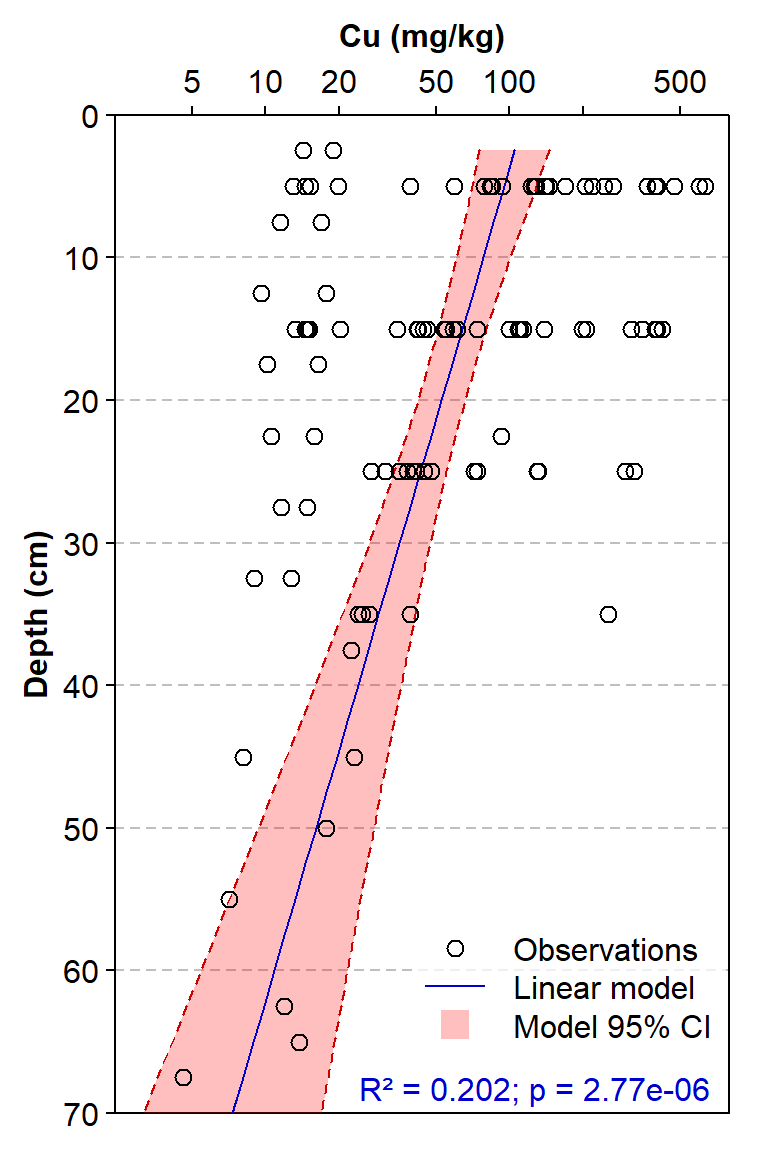

Figure 2: Depth profile of copper concentrations for multiple sediment cores, with Cu concentrations fitted to a linear model with Depth as the single predictor.

Variable as a linear function of depth – single profile

We can also apply a linear model to a single depth profile, e.g. from one sediment core or soil pit.

par(mfrow=c(1,1), mar=c(1,3,3,1), mgp=c(1.6,0.4,0), tcl=-0.2, lend="square",
    font.lab=2)
palette(c("black","blue3","red3","#ff000040","#ffffffc0","transparent"))
g10 <- droplevels(afs25[which(afs25$Group==10),])
with(g10, plot(Gd, Depth_mean, type="n", ylab="", 
                    xaxt="n", xlab="", yaxs="i", 
                    cex=1.2, xlim=c(-2,11), ylim=c(70,0), las=1, xaxt="n"))
abline(h=seq(10,60,10), lty=2, col="#00000040")
axis(3)
mtext("Gd (mg/kg)", side=3, line=1.6, font=2)
mtext("Depth (cm)", side=2, line=1.7, font=2)
lm0 <- lm(Gd~Depth_mean, data=g10)
slm0 <- summary(lm0)
depfz <- data.frame(Depth_mean = seq(2.5,70,2.5))
predz <- as.data.frame(predict(lm0, newdata = depfz, interval="confidence"))
predz <- cbind(depfz, predz)
polygon(c(predz$lwr, rev(predz$upr), predz$lwr[1]),
        c(predz$Depth_mean, rev(predz$Depth_mean),predz$Depth_mean[1]),
        col=4, border=6)
lines(predz$fit, predz$Depth_mean, col=2)
lines(predz$lwr, predz$Depth_mean, col=3, lty=2)
lines(predz$upr, predz$Depth_mean, col=3, lty=2)
with(g10, points(Gd, Depth_mean, cex=1.2, pch=19))
text(par("usr")[2],par("usr")[3],col=2,
     labels=paste0("R² = ",signif(slm0$r.sq,2), "; p = ",
                   signif(1-(pf(summary(lm0)$fst, 1, lm0$df.res)[[1]]),2),
                   "\n"), pos=2)
legend("bottomright", legend=c("Observations","Linear model","Model 95% CI"),
       pch=c(19,NA,15), pt.cex=c(1.2,NA,2), col=c(1,2,4), lwd=c(NA,1,NA),
       bg=5, box.col=6, inset=c(0.005,0.05))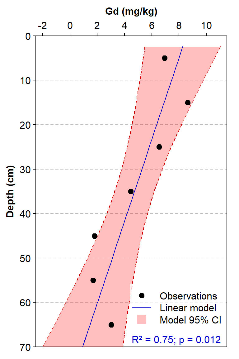

Figure 3: Depth profile of gadolinium concentrations for a single sediment core, with Gd concentrations fitted to a linear model with Depth as the single predictor.

Variable as a cubic polynomial function of depth – single profile

A linear model may not be very satisfying or appropriate for a single profile. We can adapt a linear model to fit a polynomial curve by creating columns in our data for Depth² and Depth³, and expressing our variable as a linear function of Depth, Depth², and Depth³ using multiple regression. A cubic polynomial is usually sufficient to capture any curvature.

par(mfrow=c(1,1), mar=c(1,3,3,1), mgp=c(1.6,0.4,0), tcl=-0.2, lend="square",
    font.lab=2)
palette(c("black","blue3","red3","#ff000040","#ffffffc0","transparent"))
data0 <- na.omit(afs25[which(afs25$Group==10),c("Depth_mean","Gd")])
data0$Depth2 <- data0$Depth_mean^2
data0$Depth3 <- data0$Depth_mean^3
with(data0, plot(log10(Gd), Depth_mean, col="#00000040", pch=19, ylab="", 
                 xaxt="n", xlab="", yaxs="i", 
                 cex=1.2, xlim=log10(c(1,13)), ylim=c(70,0), las=1, xaxt="n"))
abline(h=seq(10,60,10), lty=2, col="#00000040")
axis(3, at=log10(c(1,2,5,10,20,50,100,200,500)), 
     labels=c(1,2,5,10,20,50,100,200,500))
mtext("Gd (mg/kg)", side=3, line=1.6, font=2)
mtext("Depth (cm)", side=2, line=1.6, font=2)

lm3 <- lm(log10(Gd)~Depth_mean + Depth2 + Depth3, data=data0)
slm3 <- summary(lm3)
depfz <- data.frame(Depth_mean = seq(2.5,70,2.5),
                    Depth2 = seq(2.5,70,2.5)^2,
                    Depth3 = seq(2.5,70,2.5)^3)
predz <- as.data.frame(predict(lm3, newdata = depfz, interval="confidence"))
predz <- cbind(depfz, predz)
polygon(c(predz$lwr, rev(predz$upr), predz$lwr[1]),
        c(predz$Depth_mean, rev(predz$Depth_mean),predz$Depth_mean[1]),
        col="#ff000040", border="transparent")
lines(predz$fit, predz$Depth_mean, col="blue3")
lines(predz$lwr, predz$Depth_mean, col="red3", lty=2)
lines(predz$upr, predz$Depth_mean, col="red3", lty=2)
with(data0, points(log10(Gd), Depth_mean, cex=1.2, pch=19))
text(par("usr")[1],par("usr")[4],col="blue3",
     labels=paste0("\n\n\nR² = ",signif(slm3$r.sq,3), ";\np = ",
                   signif(1-(pf(summary(lm3)$fst, 1, lm3$df.res)[[1]]),3)),
     pos=4)
legend("bottomright", legend=c("Observations","Cubic model","Model 95% CI"),
       pch=c(19,NA,15), pt.cex=c(1.2,NA,2), col=c(1,2,4), lwd=c(NA,1,NA),
       bg=5, box.col=6, inset=c(0.005,0.1))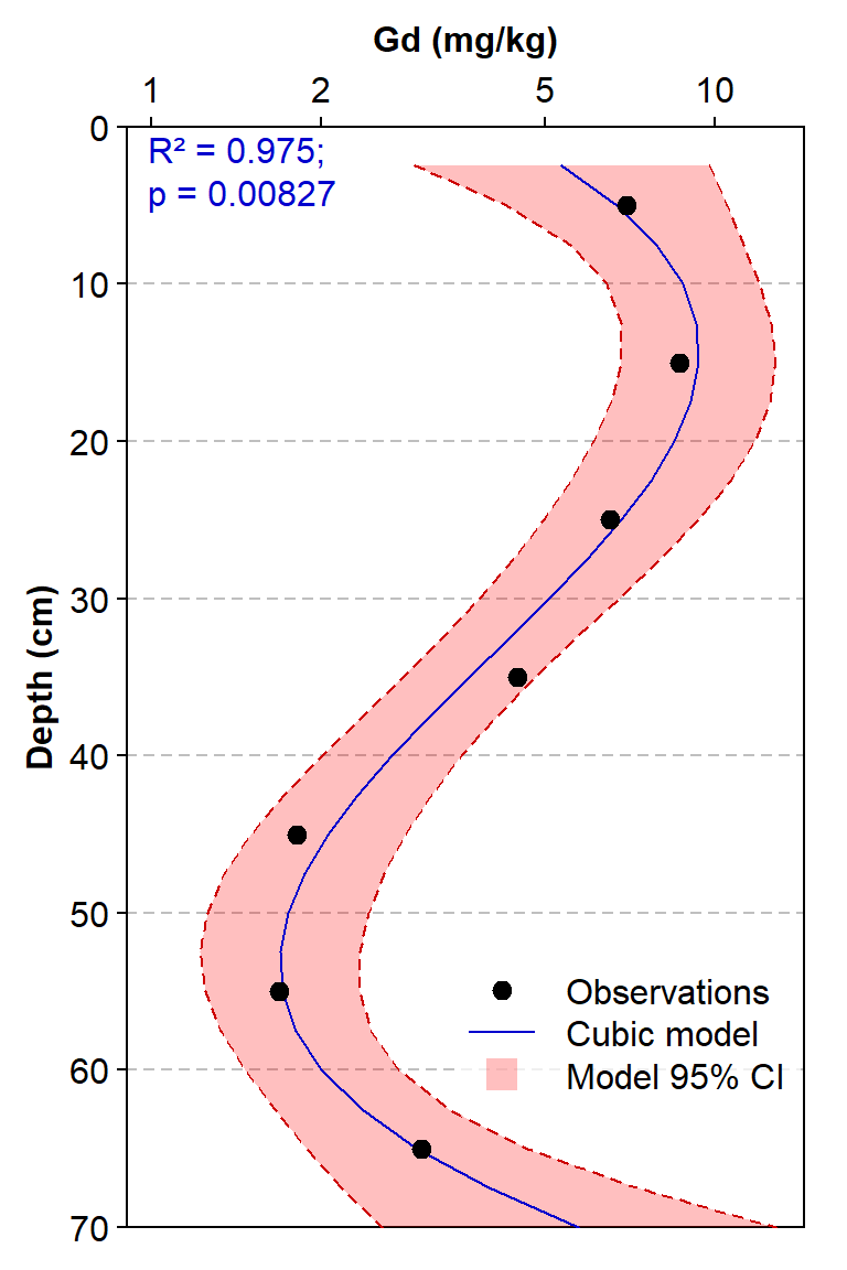

Figure 4: Depth profile of gadolinium concentrations for a single sediment core, with Gd concentrations fitted to a cubic function of Depth.

References and R Packages

Graves S, Piepho H, Dorai-Raj LSwhfS (2024). multcompView: Visualizations of Paired Comparisons. doi:10.32614/CRAN.package.multcompView, R package version 0.1-10, https://CRAN.R-project.org/package=multcompView.

Mangiafico, Salvatore S. (2024). rcompanion: Functions to Support Extension Education Program Evaluation. version 2.4.36. Rutgers Cooperative Extension. New Brunswick, New Jersey. https://CRAN.R-project.org/package=rcompanion

Snow G (2024). TeachingDemos: Demonstrations for Teaching and Learning. doi:10.32614/CRAN.package.TeachingDemos, R package version 2.13, https://CRAN.R-project.org/package=TeachingDemos.

CC-BY-SA • All content by Ratey-AtUWA. My employer does not necessarily know about or endorse the content of this website.
Created with rmarkdown in RStudio. Currently using the free yeti theme from Bootswatch.