how to boxplot
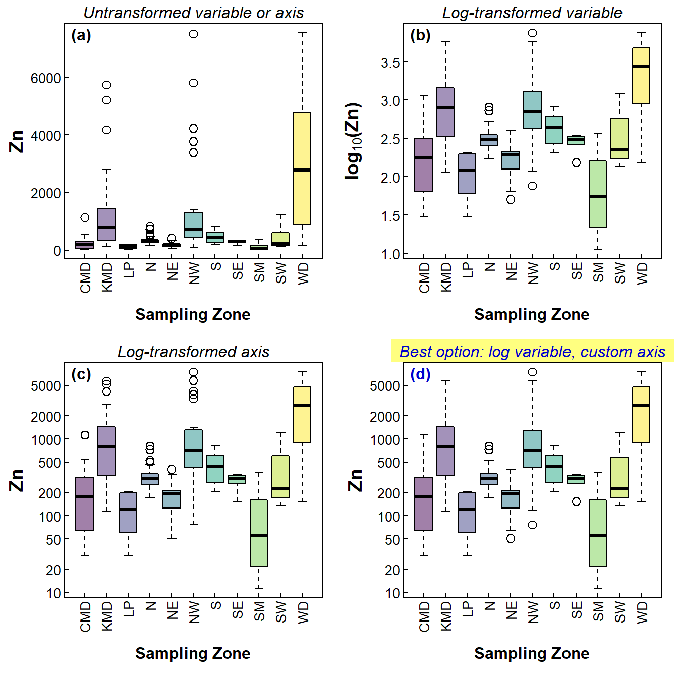
For exploratory data analysis I draw a lot of boxplots. Also, the data that I typically look at have mainly positively skewed variables. When drawing boxplots, this means that some categories can be hard to visualise because they have much lower concentrations than others, and the high values dominate the plot (see Figure 1(a)).
We usually deal with this by log transformation - Figure 1(b) shows this, and the variables (and therefore boxplot boxes) now have more symmetrical distributions which are all clearly visible on the plot. But the y axis (concentration, in this case) doesn't show the actual values.
Figure 1(c) shows the plot with a log-transformed axis scale, but this is not really satisfying either since the distribution is still skewed but plotted on the compressed log-transformed y-axis.
I think the best option, shown in Figure 1(d), is to plot the log-transformed variable, but suppress the automatic axis and manually add a y-axis with a transformed scale. It's a bit trickier, but worth it. Now we can compare all the factor levels easily, yet still have actual values on the axis (e.g. for comparison with environmental guidelines).
par(mfrow=c(2,2),mar = c(5,4,1.5,1), mgp=c(2.4,0.2,0), tcl=0.25, font.lab = 2,
    xpd = TRUE)
library(viridis)

with(afsed1922, boxplot(Zn ~ Zone, col=viridis(11, alpha=0.5),
                        las=2, xlab="", cex = 1.4, cex.lab = 1.4))
mtext("Sampling Zone",1,3,font=2)
mtext("(a)", 3, -1.2, adj = 0.03, font = 2)
mtext("Untransformed variable or axis", 3, 0.2, font=3)

with(afsed1922, boxplot(log10(Zn) ~ Zone, col=viridis(11, alpha=0.5),
                        las=2, xlab="", cex = 1.4, cex.lab = 1.4,
                        ylab=expression(bold(paste(log[10],"(Zn)")))))
mtext("Sampling Zone",1,3,font=2)
mtext("(b)", 3, -1.2, adj = 0.03, font = 2)
mtext("Log-transformed variable", 3, 0.2, font=3)

with(afsed1922, boxplot(Zn ~ Zone, log = "y", col=viridis(11, alpha=0.5),
                        las=2, xlab="", cex = 1.4, cex.lab = 1.4))
mtext("Sampling Zone",1,3,font=2)
mtext("(c)", 3, -1.2, adj = 0.03, font = 2)
mtext("Log-transformed axis", 3, 0.2, font=3)

with(afsed1922, boxplot(log10(Zn) ~ Zone, col=viridis(11, alpha=0.5),
                        las=2, xlab="", cex = 1.4, cex.lab = 1.4, yaxt="n",
                        ylab = "Zn"))
axis(2, at=log10(c(10,20,50,100,100,200,500,1000,2000,5000)),
     labels=c(10,20,50,100,100,200,500,1000,2000,5000),las=2)
mtext("Sampling Zone",1,3,font=2)
mtext("(d)", 3, -1.2, adj = 0.03, font = 2, col = "blue3")
rect(-0.5,log10(10000),12.5,log10(20000), border = NA, col = "#FFFF80")
mtext("Best option: log variable, custom axis", 3, 0.2, font=3, col = "blue3")
Figure 1: Four styles of boxplots based on the same data.
Of course, this is not the only modification we can make with box
plots. A box plot is a good way to compare the spread of values between
different levels of a factor, and the thick line inside boxes shows how
the medians in each group vary. Sometimes we also like to look at where
the mean values are, especially if we have a parametric statistical test
to compare these means. It's not too difficult to superimpose the means
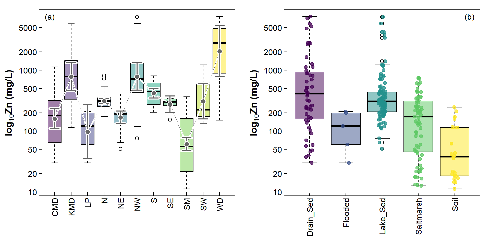
together with some measure of variability; the following example (Figure
2) shows 95% confidence intervals around each group mean. We use the
group.CI() function in the Rmisc package to
calculate confidence intervals for a variable in groups defined by a
factor.
library(Rmisc)
par(mfrow=c(1,2), mar=c(5,4,1,1), mgp=c(2.4,0.2,0), tcl=0.25, font.lab = 2, las=1)
# change data object, variable & factor names to suit your data
ci0 <- group.CI(log10(Zn)~Zone, data=afsed1922)
with(afsed1922,
     boxplot(log10(Zn) ~ Zone, col=viridis(NROW(ci0), alpha=0.5),
             ylab=expression(bold(paste(log[10],"Zn (mg/L)"))),
             cex.lab=1.2, yaxt="n", xaxt = "n", xlab = "")
     )
axis(1, las = 2, tcl = 0.4, at = seq(1,NROW(ci0)),
     labels = as.character(levels(afsed1922$Zone)))
axis(2, at=log10(c(10,20,50,100,100,200,500,1000,2000,5000)),
     labels=c(10,20,50,100,100,200,500,1000,2000,5000),las=2)
mtext("Sampling zone", side = 1, line = 5, font = 2, cex = 1.2)
#
# use arrow function to make background for [optional] error bars
arrows(x0=seq(1,NROW(ci0)), y0=ci0[,3], y1=ci0[,2],
       col="white", angle=90, length=0.1, lwd=6) # optional
arrows(x0=seq(1,NROW(ci0)), y0=ci0[,3], y1=ci0[,4],
       col="white", angle=90, length=0.1, lwd=6) # optional
#
# draw lines to join points first, so the points overplot lines
lines(seq(1,NROW(ci0)), ci0[,3], col="white", lwd=3, type="c")
lines(seq(1,NROW(ci0)), ci0[,3], col="gray40", lwd=1, type="c", lty=3)
#
# use arrow function to make actual [optional] error bars
arrows(x0=seq(1,NROW(ci0)), y0=ci0[,3], y1=ci0[,2],
       col="gray40", angle=90, length=0.1, lwd=2, lend=1)
arrows(x0=seq(1,NROW(ci0)), y0=ci0[,3], y1=ci0[,4],
       col="gray40", angle=90, length=0.1, lwd=2, lend=1)
# draw the points with white background for contrast
points(seq(1,NROW(ci0)), ci0[,3], col="white", pch=16, lwd=2, cex=1.6)
points(seq(1,NROW(ci0)), ci0[,3], col="gray40",
       pch=16, lwd=2, cex=1.2)
mtext("(a)", 3, -1.2, adj = 0.03)

nc <- nlevels(afsed1922$Type)
palette(c("black",viridis(nc, alpha=0.5),
          viridis(nlevels(afsed1922$Type), alpha=0.75),"white"))
with(afsed1922,
     boxplot(log10(Zn) ~ Type, col=c(1:nc)+1,
             ylab=expression(bold(paste(log[10],"Zn (mg/L)"))),
             cex.lab=1.2, yaxt="n", xlab = "",las=2))

axis(2, at=log10(c(10,20,50,100,100,200,500,1000,2000,5000)),
     labels=c(10,20,50,100,100,200,500,1000,2000,5000),las=2)
with(afsed1922, stripchart(log10(Zn) ~ Type, add = TRUE, vertical=TRUE,
                           method="jitter", pch=19,col=c(1:nc)+(nc+1)))
mtext("(b)", 3, -1.2, adj = 0.97)
Figure 2: Including additional information on boxplots; (a) mean and CI, (b) individual observations.
CC-BY-SA • All content by Ratey-AtUWA. My employer does not necessarily know about or endorse the content of this website.
Created with rmarkdown in RStudio using the cyborg theme from Bootswatch via the bslib package, and fontawesome v5 icons.