Introduction to Compositional Data Analysis

 See also my other GitHub Pages website dedicated to teaching: “R for Environmental Science”.

 

Preamble

This page is Part 1 of a series on Compositional Data Analysis which is a micro-credential course at The University of Western Australia. Only the first two parts are publicly available. Part 2 on Principal Components Analysis for Compositional Data is available here.

Compositional data, defined as any measurements which are proportions of some whole, are common in many disciplines, including (Table 1):

 

Compositional data have mathematical properties which result in misleading conclusions from traditional statistical analyses. Compositional variables (including concentrations of substances in water [or air, or rock, or soil, and so on] or proportions of land surface coverage) are technically part of a fixed-sum closed set. For example, with data on percent land use over an urban area, all percentages add up to 100%! As Greenacre (2018) points out, we often deal with subcompositions rather than compositions, because we do not (or can not) measure all possible components of a sample. For example, in environmental science, when we measure the substances present in water, we don't usually measure the concentration of water itself. Or in politics, we report the proportions of voters who voted for each candidate, but not often the proportion of citizens who didn't vote.

The issue of subcompositions is not necessarily a problem. For instance, in the political example above, the ratio of voters supporting the two leading candidates will be the same whether we consider the total eligible electors, or only the people who actually voted. As we will see below, a key strategy for analysing compositional data is the use of some sort of ratio.

If uncorrected, analysis of data having fixed-sum closure can lead to very misleading conclusions, especially when relationships between variables are being investigated, as in correlation analyses or multivariate methods such as principal component analysis. Closed data require specialised transformations to remove closure, such as calculation of centered or additive log ratios (Reimann et al. 2008). The centered log-ratio is defined by:

\(x_{CLR} = log(\dfrac{x}{geomean(x_{1},...,x_{n})})\), where

• \(x\) is the value being transformed (concentration, proportion);
• \(x_{CLR}\) is the centered log-ratio transformed value;
• \(geomean\) means the geometric mean of;
• \(x_{1}...x_{n}\) are all the \(n\) values contributing to the (sub)composition, including the one (\(x\)) being transformed;
• all the components (parts) of the composition need to be in identical units (e.g. percent, mg/L, incidence per 10,000, etc.).

For example, in a soil texture analysis where the proportions of grain size categories gravel (G), sand (S), silt (Z), and clay (C) all add up to 100%, the CLR-transformed sand content is:

\(S_{CLR} = log(\dfrac{S}{geomean(G,S,Z,C)})\)

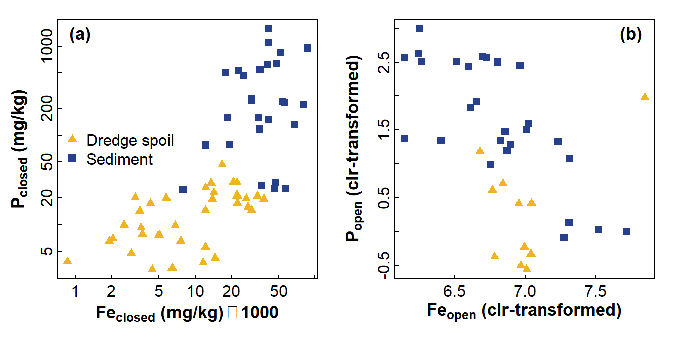
The example in Figure 1 shows the relationship between phosphorus (P) and iron (Fe) in soil/sediment materials in an acid sulfate environment. Without correcting for compositional closure, the P vs. Fe plot implies that P increases as Fe increases. Correcting for compositional closure, however, suggests the opposite, with P negatively related to Fe! In this case, if we had used conventional transformations, we might have come to a very wrong conclusion about the sediment properties affecting phosphorus.

Figure 1: Comparison of relationships between P and Fe for (a) compositionally closed concentrations showing a positive relationship and (b) concentration variables corrected for compositional closure using centred log ratios showing a negative relationship. Data from Xu et al. (2018).

 

In this UWA Micro-Credential course, you will learn specialised methods which allow you to analyse compositional data so that results can be interpreted with confidence. Students will also gain skills in use of R for relevant multivariate data analyses.

 

First we load the packages we need, and set a preferred colour palette.

library(stringr)     # manipulate character strings
library(RcmdrMisc)   # statistical functions
library(MASS)        # statistical functions
# library(rgr)       # does not work with recent R versions, no longer used
library(car)         # statistical functions focused on regression
library(cluster)     # cluster analysis
library(factoextra)  # multivariate visualisation
library(ggplot2)     # more visualisation
library(reshape2)    # data wrangling
library(ggpubr)      # arrangement of graphics from factoextra ± ggplot2

palette(c("black", "#003087", "#DAAA00", "#8F92C4", "#E5CF7E",
          "#001D51", "#B7A99F", "#A51890", "#C5003E", "#FDC596",
          "#AD5D1E", "gray40", "gray85", "#FFFFFF", "transparent"))

Load the cities data

Data are from: Fig. 11 in Hu, J., Wang, Y., Taubenböck, H., Zhu, X.X., 2021. Land consumption in cities: A comparative study across the globe. Cities, 113: 103163, https://doi.org/10.1016/j.cities.2021.103163. (digitised from figure using https://automeris.io/WebPlotDigitizer/)

[If you were hoping for an example using geochemical-type compositional data – don't worry, we're going to repeat all the analyses below using just such a dataset.]

After reading the data we make a column containing abbreviated codes for the land-use type factor, using the gsub() function to substitute character strings.

cities <-
  read.csv(paste0("https://raw.githubusercontent.com/Ratey-AtUWA/",
                  "compositional_data/main/cities_Hu_etal_2021.csv"),
           stringsAsFactors = TRUE)
flextable(cities) |>
  width(j=1:8, width=c(2.7,1.5,1.5,1.8,1.5,3,2,3), unit = "cm") |>
  add_header_row(values = c("","Land use categories","City categories"),
                     colwidths = c(1,4,3)) |>
  set_caption(caption = "Table 2: Cities land use data used in this document, showing cities categorized by land-use Type, Global socioeconomic zone, and geographic Region.") |>
  theme_zebra(odd_header = "#D0E0FF", even_header = "#D0E0FF") |>
  align(align = "center", part = "header") |>
  height_all(height=0.39, unit = "cm") |>
  hrule(rule = "exact") |>
  border_outer(border = BorderDk, part = "all") |>
  border_inner_v(border=BorderLt, part="header")

 

The original data categorised the cities by Type, based on the land use categories occupying the greatest proportion(s) of urban area. We have added two other categories, Global identifying each city as being in the socioeconomic "global south" or "global north" zones, and also assigning each city to a geographic Region, a category having eight levels. All categories are stored as factors in the R data frame.

Make CLR-transformed dataset

cities_clr <- cities
cities_clr[,2:5] <- t(apply(cities[,2:5], MARGIN = 1,
                           FUN = function(x){log(x) - mean(log(x))}))
head(cities_clr[,1:8])

##                City  Compact      Open Lightweight Industry         Type Global        Region
## New York   New York 2.784665  3.318548   -8.234636 2.131422 Compact-Open  North North America
## Sao Paulo Sao Paulo 3.464227  2.870435   -8.164132 1.829470 Compact-Open  South South America
## Shanghai   Shanghai 1.590463  3.203702   -8.126454 3.332290   Industrial  South  Eastern Asia
## Beijing     Beijing 2.721094  3.370144   -8.181002 2.089764 Compact-Open  South  Eastern Asia
## Jakarta     Jakarta 4.275083 -0.300825   -7.416407 3.442149      Compact  South    South Asia
## Guangzhou Guangzhou 3.113608  1.827387   -8.094137 3.153142      Compact  South  Eastern Asia

Compare correlation matrices

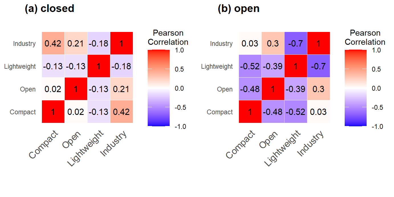
Figure 2: Correlation matrices for (a) closed, and (b) open (CLR-transformed) variables (code is not shown).

 

By comparing Figure 2(a) and Figure 2(b), we can already see that addressing closure with the centered-logratio (CLR) transformation changes the interpretation of relationships between the variables.

Some other things to try comparing the distributions of untransformed and CLR-transformed pairs of variables using histograms or density plots comparing scatter plots of untransformed and CLR-transformed pairs of variables (maybe using the scatterplotMatrix() function in the car package).

 

---

Load some geochemical data

Data edited from: Rate & McGrath (2022a) (described in Rate & McGrath, 2022b).

ashfield <-
  read.csv(paste0("https://raw.githubusercontent.com/Ratey-AtUWA/",
                  "compositional_data/main/AFR_surfSed_2019-2021.csv"),
           stringsAsFactors = TRUE)
ashfield$Year <- as.factor(ashfield$Year)
flextable(ashfield[seq(1,100,8),c(1,2,4,7,8,9:17)]) |>
  set_caption(caption = "Table 3: Selection of 12 rows and 14 columns of a dataset of chemical compositions for sediments samples at Ashfield Flats Reserve, 2019-2021.") |>
  theme_zebra(odd_header = "#D0E0FF", even_header = "#D0E0FF") |>
  align(align = "center", part = "header") |>
  height_all(height=0.39, unit = "cm") |>
  hrule(rule = "exact") |>
  border_outer(border = BorderDk, part = "all") |>
  border_inner_v(border=BorderLt, part="header")

 

We notice from Table 3 that there are both non-compositional variables (e.g. coordinates, pH, EC) and compositional variables (e.g. Al, As, Ba, Ca, Ce, Co). We also have missing data shown by the blank cells in Table 3 (these are NA in the R data frame).

Make CLR-transformed geochemical dataset

We only transform the set of closed compositional variables. Note that we need to include the argument na.rm=TRUE in the mean() function applied, since our dataset has missing values.

ashfield_clr <- ashfield
ashfield_clr[,11:38] <- t(apply(ashfield[,11:38], MARGIN = 1,
                           FUN = function(x){log(x) - mean(log(x), na.rm=TRUE)}))
head(ashfield_clr[,11:17])

##         Al        As         Ba       Ca        Cd         Ce        Co
## 1 4.915247 -2.629041 -0.9121439 4.363272 -5.860602 -1.7556753 -0.808294
## 2 5.485119 -3.237030 -0.8175805 3.059425 -5.505493 -0.5044887 -2.056470
## 3 5.453100 -3.673684 -0.8895440 3.585314 -6.701993 -0.4096881 -2.581503
## 4 5.510806        NA -0.3797352 3.032430 -7.305800 -0.5253843 -2.722609
## 5 5.601512 -2.808624 -0.6332189 3.276841 -7.804974 -0.3297310 -2.845259
## 6 5.774326 -3.398333 -0.5061159 3.665076 -8.188598 -0.3984539 -2.680560

Compare correlation matrices (geochemical data)

We include pH and EC in the correlation matrix as well as the set of compositionally closed compositional variables. Note that we need to include the argument use="pairwise.complete.obs" in the cor() function, as this will maximise use of a dataset with missing values.

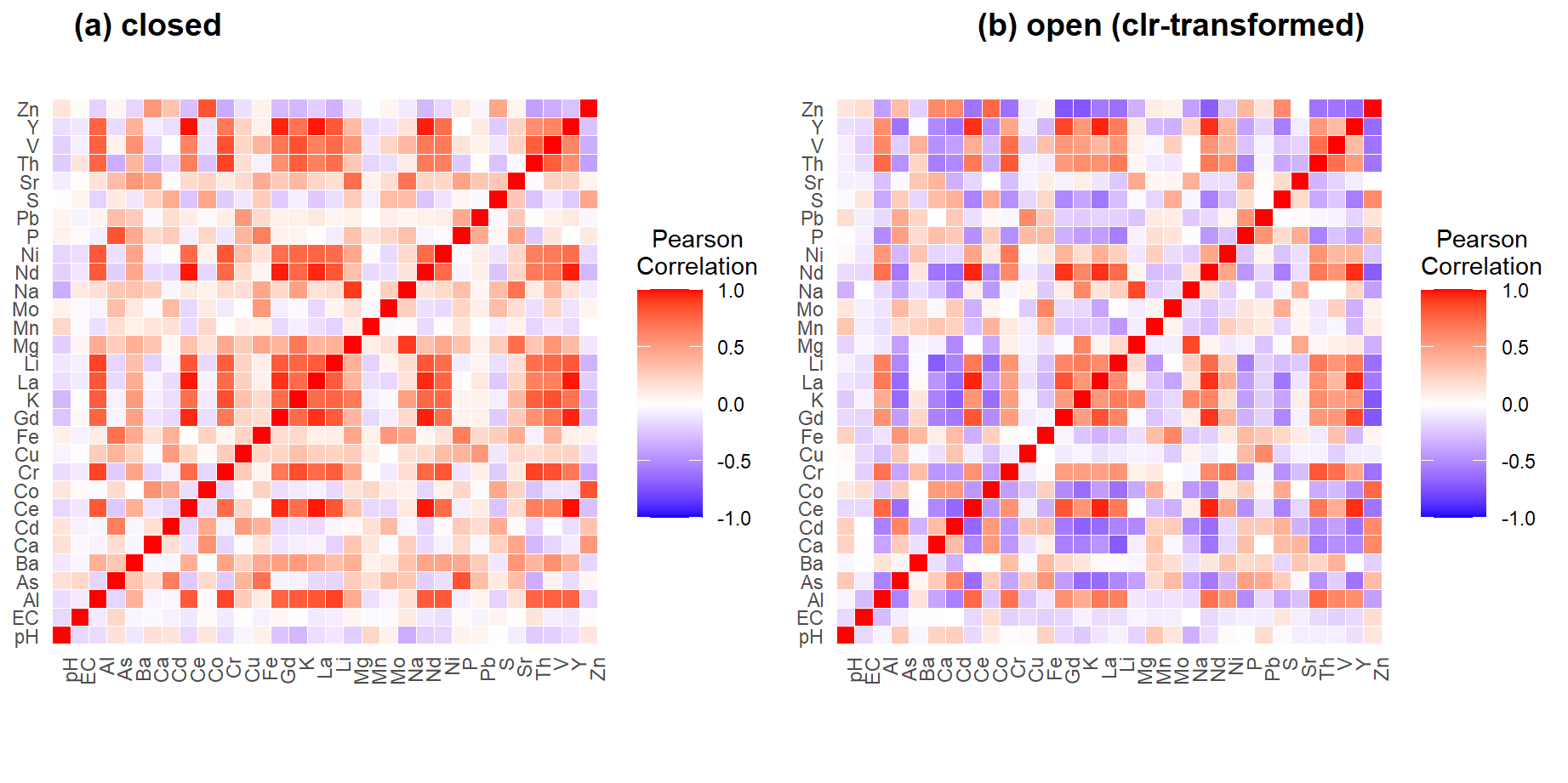
Figure 3: Correlation matrices for (a) closed, and (b) open (CLR-transformed) variables in the geochemical dataset (code is not shown).

 

By comparing Figure 3(a) and Figure 3(b), we can see again, as for the Cities data (Figure 2), that addressing compositional closure with the centered-logratio (CLR) transformation changes the interpretation of relationships between the variables.

In the next sessions we will apply more sophisticated multivariate statistical methods to analysis of data having fixed-sum compositional closure. These methods include ordinations such as principal components analysis (PCA), different types of cluster analysis, and classification methods such as linear discriminant analysis (LDA).

---

Link to Part 2 on Principal Components Analysis for Compositional Data

---

 

References and R Packages

Fox, J. (2022). RcmdrMisc: R Commander Miscellaneous Functions. R package version 2.7-2. https://CRAN.R-project.org/package=RcmdrMisc

John Fox and Sanford Weisberg (2019). An {R} Companion to Applied Regression (car), Third Edition. Thousand Oaks CA: Sage. URL: https://socialsciences.mcmaster.ca/jfox/Books/Companion/

Greenacre, M. (2018). Compositional Data Analysis in Practice. CRC Press LLC, Boca Raton, FL, USA.

Hu, J., Wang, Y., Taubenböck, H., Zhu, X.X. (2021). Land consumption in cities: A comparative study across the globe. Cities, 113: 103163, doi:10.1016/j.cities.2021.103163.

Kassambara, A. and Mundt, F. (2020). factoextra: Extract and Visualize the Results of Multivariate Data Analyses. R package version 1.0.7. https://CRAN.R-project.org/package=factoextra

Maechler, M., Rousseeuw, P., Struyf, A., Hubert, M., Hornik, K.(2021). cluster: Cluster Analysis Basics and Extensions. R package version 2.1.2. https://CRAN.R-project.org/package=cluster

Rate, A.W., & McGrath, G. (2022a). Sediment and soil quality at Ashfield Flats Reserve, Western Australia (Version 1). Mendeley Data, doi:10.17632/d7m3746byk.1

Rate, A. W., & McGrath, G. S. (2022b). Data for assessment of sediment, soil, and water quality at Ashfield Flats Reserve, Western Australia. Data in Brief, 41, 107970. doi:10.1016/j.dib.2022.107970

Reimann, C., Filzmoser, P., Garrett, R. G., & Dutter, R. (2008). Statistical Data Analysis Explained: Applied Environmental Statistics with R (First ed.). John Wiley & Sons, Chichester, UK.

Venables, W. N. & Ripley, B. D. (2002) Modern Applied Statistics with S (MASS). Fourth Edition. Springer, New York. ISBN 0-387-95457-0. http://www.stats.ox.ac.uk/pub/MASS4/

Wickham, H. (2019). stringr: Simple, Consistent Wrappers for Common String Operations. R package version 1.4.0. https://CRAN.R-project.org/package=stringr

Xu, N., Rate, A. W., & Morgan, B. (2018). From source to sink: Rare-earth elements trace the legacy of sulfuric dredge spoils on estuarine sediments. Science of The Total Environment, 637-638, 1537-1549, doi:10.1016/j.scitotenv.2018.04.398.

---

CC-BY-SA • All content by Ratey-AtUWA. My employer does not necessarily know about or endorse the content of this website.
Created with rmarkdown in RStudio using the cyborg theme from Bootswatch via the bslib package, and fontawesome v5 icons.