Read data from Hydrus-1D
nod_inf.out files
Users of Hydrus-1D either need to use the limited graphics in
Hydrus itself, open the output files in Excel, or figure out a way of
using more flexible software. So here's my code to read the node
(Profile) information output files from Hydrus-1D
(Nod_Inf.out in the relevant Hydrus-1D project folder) into
an R data frame.
# R code to read Hydrus-1D Nod_Inf.out files into an R data frame
# set full path to Hydrus-1D project directory (folder)
# -=-=-=-=- EDIT THIS TO MATCH THE FOLDER ON YOUR COMPUTER ! -=-=-=-=-
PCdir <- paste0(MyPC,"My Documents/aaTeaching/ENVT5503/Hydrus1D ENVT5503/PRB")
# read Nod_Inf.out file into a vector of character (text) strings
Nod_Inf_out <- readLines(paste0(PCdir,"/","Nod_Inf.out"))
# View(Nod_Inf_out) # optionally check what we just read
# find indices of some rows we want to delete
head_rows <- grep("Node", Nod_Inf_out)
# use indices to delete the rows
Nod_Inf_out <- Nod_Inf_out[-c(seq(1,7),head_rows-2, head_rows-1,
                              head_rows+1, head_rows+2)]
# find indices of some more rows we want to delete
ends <- grep("end",Nod_Inf_out)[-1*NROW(grep("end",Nod_Inf_out))]
# use indices to delete the rows
Nod_Inf_out <- Nod_Inf_out[-c(ends, ends+1, ends+2)]
# find indices of rows that have the Hydrus-1D print times
time_rows <- grep("Time:", Nod_Inf_out)
# extract the rows with Hydrus-1D print times into a vector
timz <- Nod_Inf_out[time_rows]
# get rid of text around the Hydrus-1D print time values...
timz <- gsub("Time: ","",timz)
timz <- gsub(" ","",timz)
# ...and convert to numbers...
timz <- as.numeric(timz)
# ...then delete the Hydrus-1D print time rows
Nod_Inf_out <- Nod_Inf_out[-c(time_rows)]
# find the rows with column names for each block of print data...
head_rows <- grep("Node", Nod_Inf_out)
# and remove all except the first one
Nod_Inf_out <- Nod_Inf_out[-c(head_rows[-1])]
# strip out all but single spaces from data...
while(NROW(grep("  ", Nod_Inf_out)) > 0) {
  Nod_Inf_out <- gsub("  "," ", Nod_Inf_out)
}
# ...and (finally!) delete the very last row (an 'end' statement)
Nod_Inf_out <- Nod_Inf_out[-1*NROW(Nod_Inf_out)]
#
# write the edited output to a file...
writeLines(Nod_Inf_out, con="./NodInf3.out")
# ...and read the file in as space-delimited
node_data <- read.table(file = "NodInf3.out", header = TRUE, sep = " ")
# the is a blank column 1; rename it to "Time"
colnames(node_data)[1] <- "Time"
# use the print times vector to make a vector with
# the relevant time repeated for each block
timz0 <- rep(timz[1], NROW(node_data)/NROW(timz))
for (i in 2:NROW(timz)) {
  timz0 <- append(timz0, rep(timz[i], NROW(node_data)/NROW(timz)))
}
# replace the Time colum with the vector we just made...
node_data$Time <- timz0
# ...and convert Time to a factor
node_data$Time <- as.factor(node_data$Time)
# remove temporary objects...
rm(list = c("i","head_rows","Nod_Inf_out","timz","timz0","ends"))
# ...and check the cleaned-up data
str(node_data)
## 'data.frame': 707 obs. of 14 variables:
## $ Time : Factor w/ 7 levels "0","80","160",..: 1 1 1 1 1 1 1 1 1 1 ...
## $ Node : int 1 2 3 4 5 6 7 8 9 10 ...
## $ Depth : num 0 -20 -40 -60 -80 -100 -120 -140 -160 -180 ...
## $ Head : num 0 0 0 0 0 0 0 0 0 0 ...
## $ Moisture : num 0.43 0.43 0.43 0.43 0.43 0.43 0.43 0.43 0.43 0.43 ...
## $ K : num 25 25 25 25 25 ...
## $ C : num 0 0 0 0 0 0 0 0 0 0 ...
## $ Flux : num -2.5 -2.5 -2.5 -2.5 -2.5 ...
## $ Sink : num 0 0 0 0 0 0 0 0 0 0 ...
## $ Kappa : int -1 -1 -1 -1 -1 -1 -1 -1 -1 -1 ...
## $ v.KsTop : num -0.1 -0.1 -0.1 -0.1 -0.1 -0.1 -0.1 -0.1 -0.1 -0.1 ...
## $ Temp : num 20 20 20 20 20 20 20 20 20 20 ...
## $ Conc.1..NS. : num 0 0 0 0 0 0 0 0 0 0 ...
## $ Sorb.1...NS.: num 0 0 0 0 0 0 0 0 0 0 ...Plot concentration vs depth
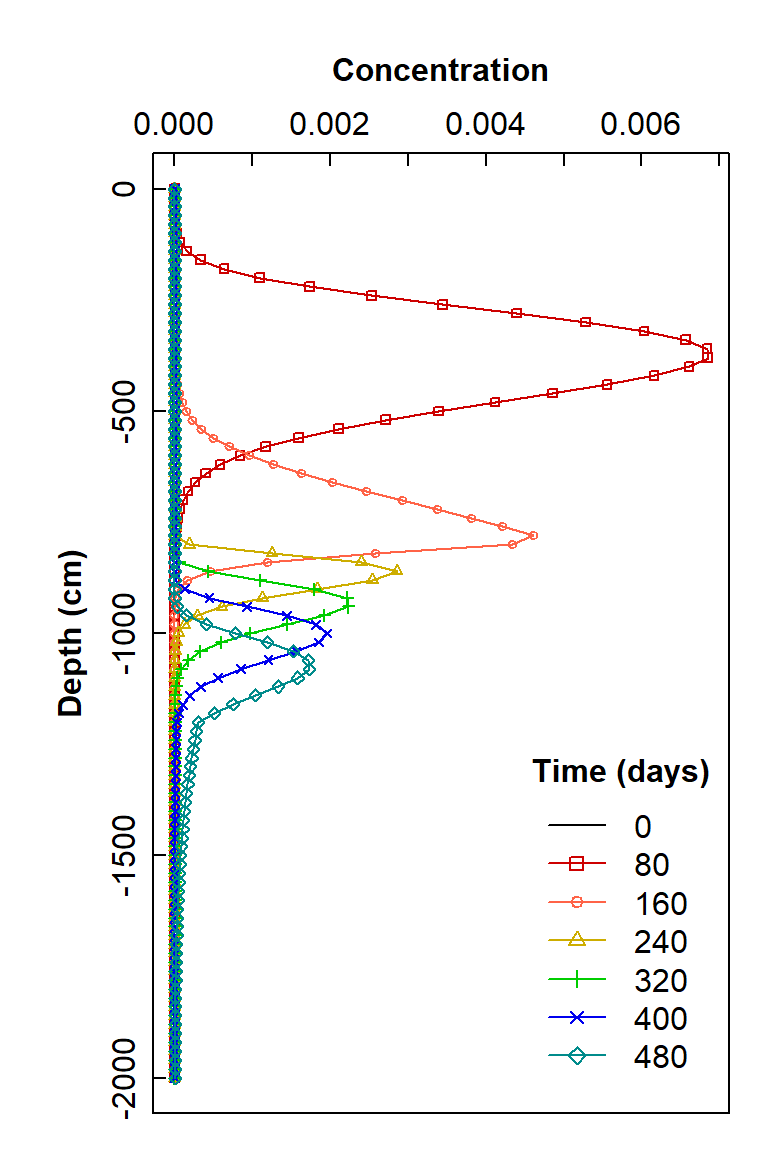
# check it with a plot
# plot as concentration vs. depth
palette(c("black","red3","tomato","gold3","green3",
         "blue2","darkcyan", "purple","sienna","gray67"))
par(mar = c(1,4,4,1), mgp = c(1.7,0.3,0), tcl = 0.3, font.lab=2)
plot(node_data$Depth ~ node_data[,13],
     type = "l", col = 1,
     xlim = c(0, max(node_data[,13], na.rm=T)),
     ylim = c(min(node_data$Depth, na.rm=T), 0),
     subset = node_data$Time==levels(node_data$Time)[1],
     xaxt = "n", xlab = "", ylab = "Depth (cm)")
axis(3)
mtext("Concentration", side = 3, line = 1.7, font = 2)
for (i in 2:nlevels(node_data$Time)) {
points(node_data$Depth ~ node_data[,13], col = i,
       subset = node_data$Time==levels(node_data$Time)[i],
       type = "o", pch = i-2, cex = 0.6)
}
legend("bottomright", legend = levels(node_data$Time),
       col = seq(1,nlevels(node_data$Time)),
       pch = c(NA,seq(0,nlevels(node_data$Time))),
       lwd = 1,
       pt.cex=0.85, bty = "n", inset = 0.02,
       title = expression(bold("Time (days)")))
Figure 1: Plot of simulated solute concentration vs. vertical depth for each simulation time step, using Hydrus-1D
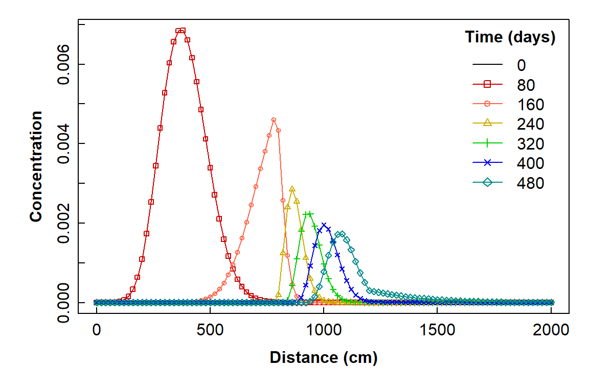
plot as concentration vs. horizontal distance
par(mar = c(4,4,1,1), mgp = c(1.7,0.3,0), tcl = 0.3, font.lab=2)
node_data$Distance <- -1*node_data$Depth
plot(node_data[,13] ~ -1*node_data$Distance,
     type = "l", col = 1,
     ylim = c(0, max(node_data[,13], na.rm=T)),
     xlim = c(0, max(node_data$Distance, na.rm=T)),
     subset = node_data$Time==levels(node_data$Time)[1],
     ylab = "Concentration", xlab = "Distance (cm)")
for (i in 2:nlevels(node_data$Time)) {
  points(node_data[,13] ~ -1*node_data$Distance, col = i,
         subset = node_data$Time==levels(node_data$Time)[i],
         type = "o", pch = i-2, cex = 0.6)
}
legend("topright", legend = levels(node_data$Time),
       col = seq(1,nlevels(node_data$Time)),
       pch = c(NA,seq(0,nlevels(node_data$Time))),
       lwd = 1,
       pt.cex=0.85, bty = "n", inset = 0.02,
       title = expression(bold("Time (days)")))
Figure 2: Plot of simulated solute concentration vs. horizontal distance for each simulation time step, using Hydrus-1D
CC-BY-SA • All content by Ratey-AtUWA. My employer does not necessarily know about or endorse the content of this website.
Created with rmarkdown in RStudio using the cyborg theme from Bootswatch via the bslib package, and fontawesome v5 icons.