Introduction

A lot of spatial information is most readily available in shapefile format, which was developed by ESRI for GIS software. The sf R package can convert shapefiles to its own object class using the versatile st_read() function.

A good source of shapefile information relevant to classes at The University of Western Australia is the dataWA portal at https://www.data.wa.gov.au/.

Downloading shapefile data from `data.wa.gov.au`

To download some of the files, you may need to register for SLIP (Shared Location Information Platform).

Stepwise procedure

We search in the portal for what we want to find (this example is for an acid sulfate soil risk map)
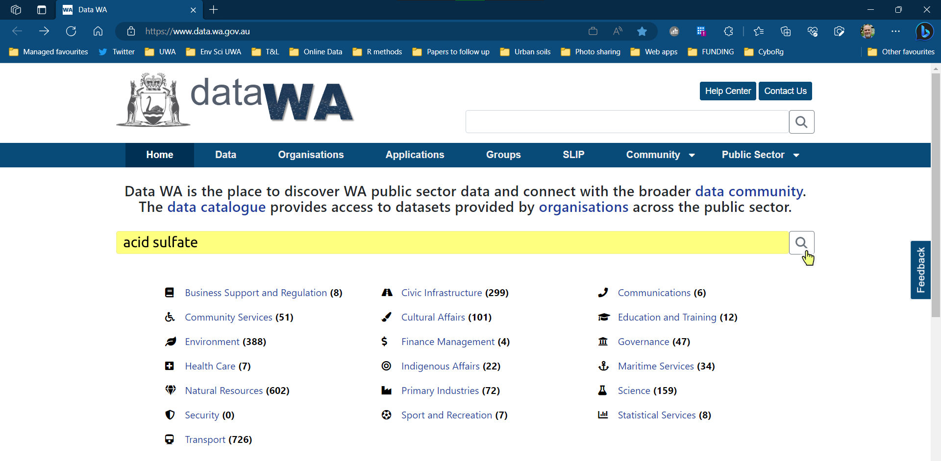
The search results list will tell us if a shapefile is available (SHP)
Open the Data Downloads section and click on ⬇Download
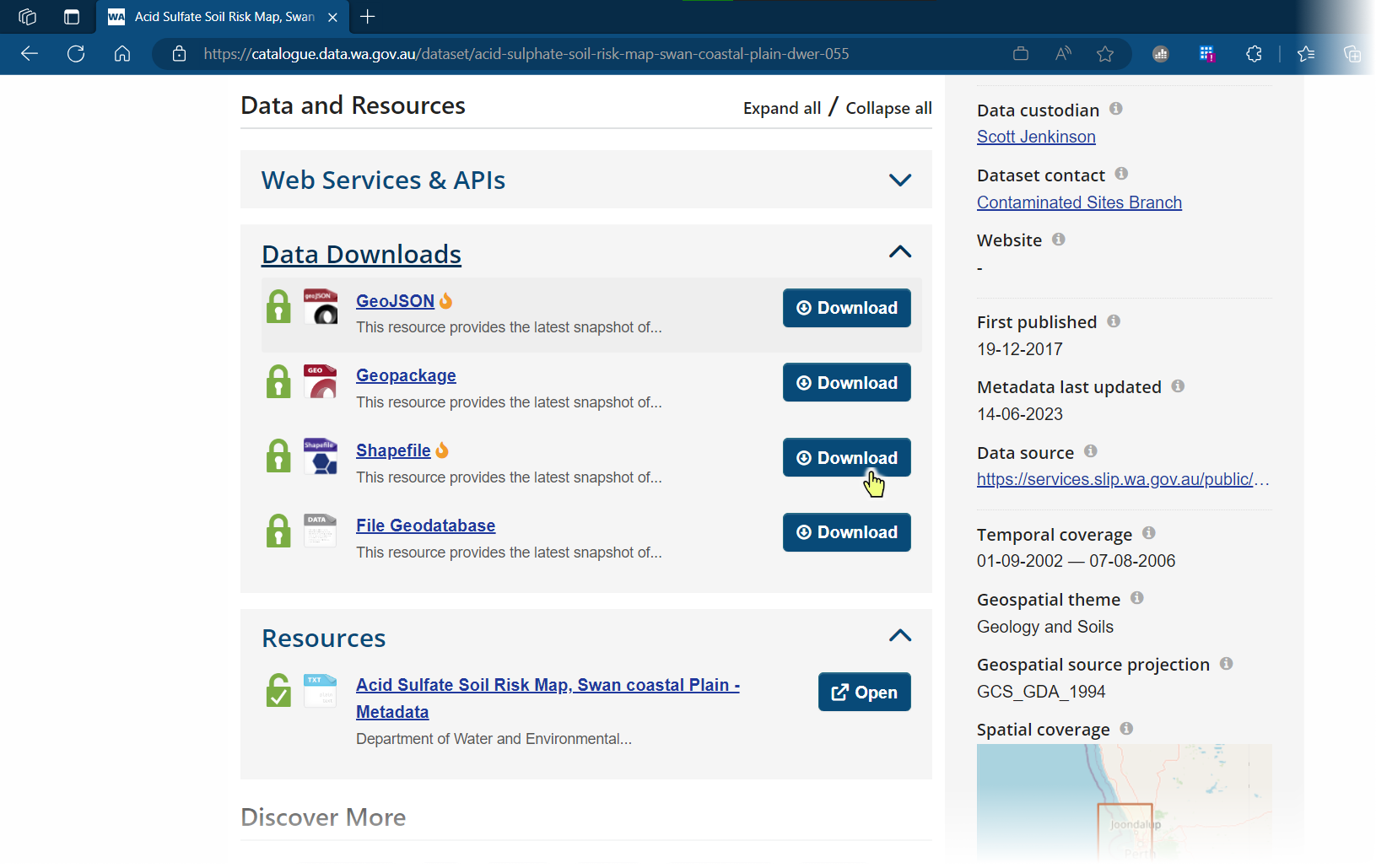
This takes us to the relevant SLIP page – click on ⬇Download again
Hover over the browser downloads and click on the folder icon
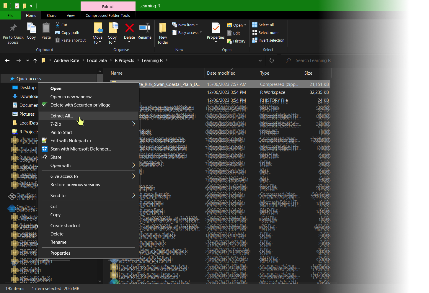
Opposite-click on the downloaded zip file and select 'Extract all' (or equivalent)
Edit the destination folder to your R working directory
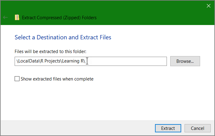
Note that you will extract several files – you need them all.

Converting the saved shapefiles for use in R

First we load any packages we need:

library(sf)
library(maptiles)
library(prettymapr)

The sf package (Pebesma 2018) function st_read() can handle many types of input file, including ESRI shapefiles.

The sf object produced will reflect the type of information in the shapefile, such as points, lines, polygons, etc.

assrisk <- 
  st_read("Acid_Sulfate_Risk_Swan_Coastal_Plain_DWER_055.shp")

## Reading layer `Acid_Sulfate_Risk_Swan_Coastal_Plain_DWER_055' from data source 
##   `C:\Users\00028958\OneDrive - The University of Western Australia\R Projects\cybloRg\Acid_Sulfate_Risk_Swan_Coastal_Plain_DWER_055.shp' 
##   using driver `ESRI Shapefile'
## Simple feature collection with 46 features and 9 fields
## Geometry type: MULTIPOLYGON
## Dimension:     XY
## Bounding box:  xmin: 114.9922 ymin: -33.74887 xmax: 116.0928 ymax: -31.24877
## Geodetic CRS:  GDA94

We should note that we only need to specify the file with extension .shp, and st_read will find the other files for us if they are in the same directory.

Plotting the converted shapefile directly

We can just use plot() to display the spatial information in the sf object created from the shapefile. Since there may be several data layers, use [] to plot them one at a time (you can check that layer 4 contains risk category information using str(assrisk)):

par(oma=c(0,0,1,8),xpd=T)
plot(assrisk[4], pal=c("orchid","gold"))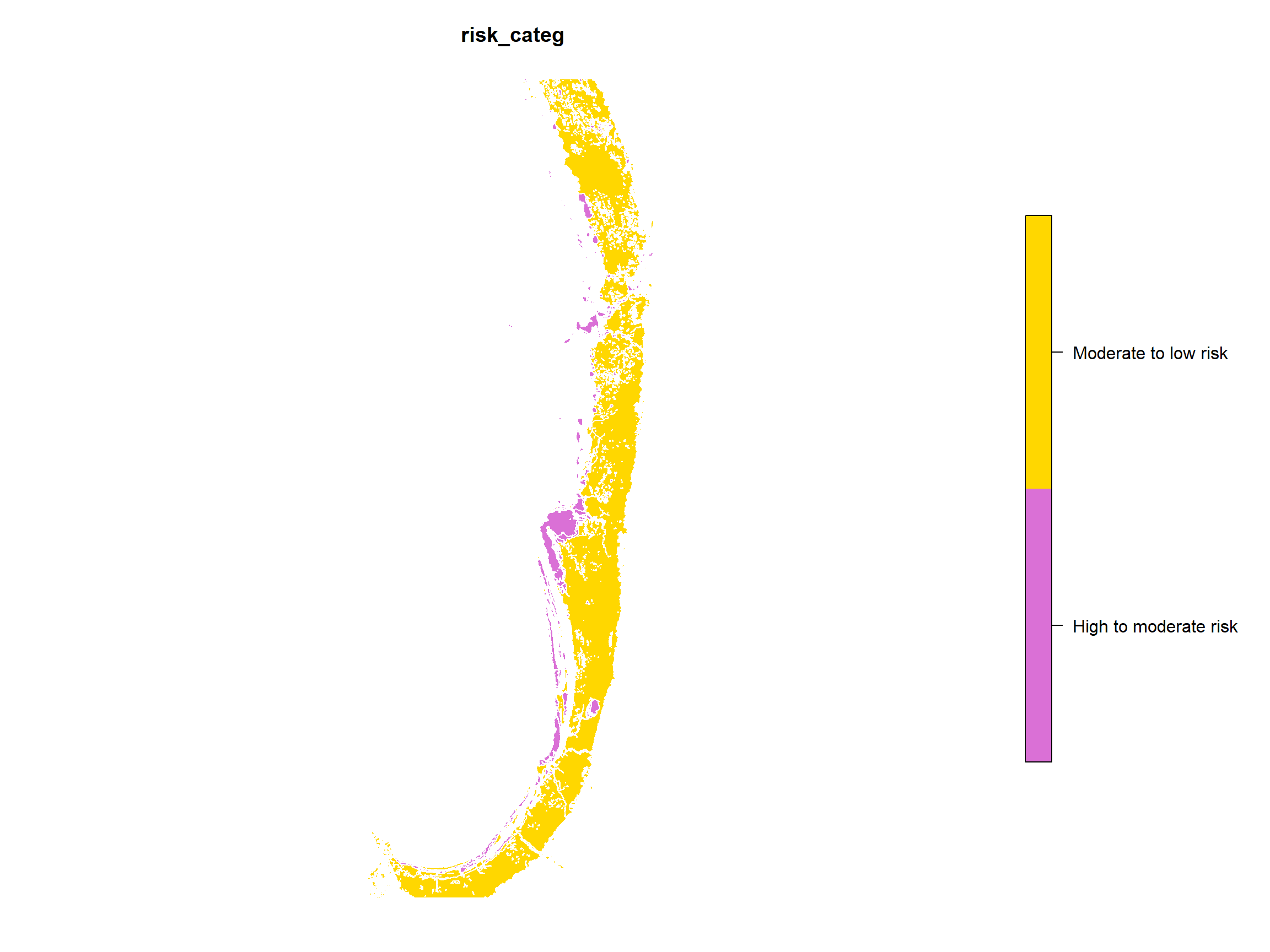

Figure 1: Plot of layer 4 in Swan Coastal Plain Acid Sulfate Soil Risk Map (DWER 2020) converted from shapefile into sf object in R.

We might notice here that the shapefile we downloaded covers the whole of the Swan Coastal Plain in Western Australia. Usually we'd like to overlay this data on a map of a smaller area. We make a sf object and use that to define a map extent for a maptiles map (Giraud 2022), and also to use st_crop() to crop the original shapefile extent to our desired area. The results are in Figure 2 below.

area <- st_as_sf(data.frame(x=c(388000,389300), y=c(6460400,6461800)),
                 coords = c("x","y"), crs=st_crs(32750))
# area_ass <- st_transform(area, crs=st_crs(assrisk))
ass_crop <- st_crop(assrisk, st_as_sf(data.frame(x=c(115.8,115.83), y=c(-32,-31.96)),
                 coords = c("x","y"), crs=st_crs(4283)))
ass_crop <- st_transform(ass_crop, crs=st_crs(32750)) # convert to UTM Zone 50S
map1 <- get_tiles(area, zoom=15, provider = "Stamen.TonerLite")
par(oma=c(3,3,1,1),mgp=c(1.6,0.3,0))
plot_tiles(map1)
axis(1,mgp=c(1.6,0.3,0));axis(2,mgp=c(1.6,0.45,0))
mtext("Easting (m)", 1, 1.6, cex=1.2,font=2)
mtext("Northing (m)", 2, 1.6, cex=1.2,font=2)
text(388370,6461200,labels="The\nUniversity\nof\nWestern\nAustralia", font=3)
text(389000,6461250,labels="Matilda\nBay", font=3)
plot(ass_crop[4], add=TRUE, pal=c("#FF808080","#FFE00040"), 
     border=c("orchid","gold3"))
addscalebar(plotepsg = 32750, pos = "bottomright", label.cex = 1.2)
addnortharrow()
legend("topleft", legend=c("Low to Moderate ASS Risk",
                           "Moderate to High ASS Risk"),
       box.col="grey62", pch=22, pt.cex=3, pt.bg=c("#FFE00040","#FF808080"),
       col=c("gold3","orchid"), cex = 1.2, inset=0.02, y.intersp = 1.2)
legend("bottomleft",legend="Datum: WGS84; EPSG:32750 (UTM Zone 50S)",cex=0.8,
       bg="white", box.col="grey64");box()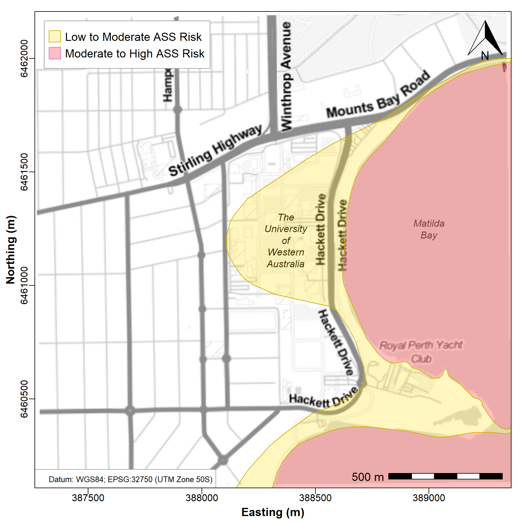

Figure 2: Map of the University of Western Australia precinct with overlay of the Swan Coastal Plain Acid Sulfate Soil Risk Map (DWER 2020). Overlay shows risk of ASS occurring in upper 3m if disturbed (e.g. by land development). Background map tiles are TonerLite (Stamen Design, 2012) via maptiles.

Packages and References

Department of Water and Environmental Regulation (DWER) (2020). Acid Sulfate Soil Risk Map, Swan Coastal Plain. Government of Western Australia, Perth. https://catalogue.data.wa.gov.au/dataset/acid-sulphate-soil-risk-map-swan-coastal-plain-dwer-055.

Giraud T (2022). maptiles: Download and Display Map Tiles. R package version 0.4.0, https://CRAN.R-project.org/package=maptiles.

Pebesma, E., 2018. Simple Features for R: Standardized Support for Spatial Vector Data. The R Journal 10 (1), 439-446, doi:10.32614/RJ-2018-009.

Stamen Design (2023) Stamen Blog > Just The Streets, Ma'am. https://stamen.com/just-the-streets-maam-f423fd694674/.

CC-BY-SA • All content by Ratey-AtUWA. My employer does not necessarily know about or endorse the content of this website.
Created with rmarkdown in RStudio using the cyborg theme from Bootswatch via the bslib package, and fontawesome v5 icons.

Using GIS shapefiles in R